Have you ever wondered how garbage collectors visit thousands of homes all over a city in a single day? Or how Pos Malaysia delivers packages so efficiently?
Ahmad is working for Pos Malaysia as a delivery man. Every morning, he starts at a depot with his delivery van, and receives a set of 17 stops in average, to deliver parcels. He needs to identify the shortest route that visits each stop once before returning to the depot.
Navigation apps like Waze are fantastic to go from point A to point B. You can also add stops in the middle, but the application won’t help you find the right order for the stops. The stength of navigation apps lies in the real-time traffic data it gathers from users, which affects the driving directions it provides.
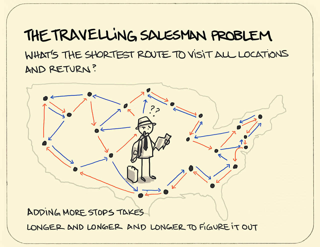
The travelling salesman problem

The travelling salesman problem (TSP) involves finding the shortest route to visits each stop once before returning to the starting point.
An obvious approach to solving the TSP is to determine all the possible routes and pick the shortest one. So why don’t people do this all the time? It turns out that this process, known as enumeration, is only feasible for very small problems.
Mathematically, suppose you have n stops, after choosing 1st starting stop arbitrarily, you have n-1 option to choose 2nd stop. And after you choose 2nd stop you have n-2 options to choose 3rd stop and so on. The number of possible routes is the factorial growth rate of the number of stops n. Total combination resulting = n-1 * n-2 * n-3 ……1 = (n-1)!
Suppose that Ahmad makes only 17 stops everyday and that he could evaluate a billion computations per second using the brute-force approach, it would take 4 days. This grows greatly as n increased and become impractical even for 20 stops, which will take 77 years.
Here is a table to show the total time taken to solve the TSP for different numbers of stops.
| Problem size (stops) | Approximate solution time |
|---|---|
| 10 | 3 mili-seconds |
| 17 | 4 days |
| 20 | 77 years |
| 25 | 490 million years |
| 30 | 8.4 x 10^15 years |
| 50 | 9.6 x 10^47 years |
As we can observe, the solution time gets out of control almost immediately, even with modest network sizes.
That’s for just one delivery man. Working stimultaneously are Ahmad’s colleagues, like Chee Ming, Muthu and 1000 more delivery men. We’re not even considering the business-specific constraints found in real problems yet. Just to name a few: multiple vehicles with limited capacity, multiple depots, vehicle limitations, cost controls, time windows, fractional loads, stochastic demands, resource limitations and heterougenous fleets.
If Pos Malaysia could make their routes just 1% more efficient, the overall savings would scale up significantly.
Miller-Tucker-Zemlin (MTZ) formulation
The TSP may be formulated as an integer linear programming (ILP) model. In the following, we develop the well known Miller-Tucker-Zemlin (MTZ) formulation. Although it is not the most computationally efficient, it is one of the easiest to code.
Label the stops enumerated as 1 … n in which n is the total number of stops and arbitrarily assume 1 as the origin.
Define the decisions variables:
x_{ij} = \begin{cases}
1  & \text{if the route includes a direct link between stops i and j} \\
0 & \text{otherwise}
\end{cases}
In addition, for each stop i = 1, 2, …, n, let u_i∈R+ be an auxiliary variable and let c_{ij} be the distance between stops i and j.
The MTZ formulation to the TSP is the following:
The objective function is then given by
\min \displaystyle\sum_{i=1}^n \displaystyle\sum_{j=1}^n c_{ij} x_{ij}To ensure that the result is a valid tour, several contraints must be added.
subject to
\begin{aligned}
& \sum_{i=1,\ j=1}^n x_{ij} = 1 & (1)\\
& \sum_{j=1,\ j=1}^n x_{ij} = 1 & (2)\\
& u_i + x_{ij} \leq u_j + (n-1) * (1 - x_{ij}) \quad 2 \leq j \leq n  & (3)\\
\\
& u_i \in \mathbb{R}^+ & (4)\\
& x_{ij} \in \{0,1\} & (5)
\end{aligned}
In the formulation above, notice that
(1) Go-to constraints: the first set of equalities requires that each stop is arrived at from exactly one other stop.
(2) Come-from constraints: the second set of equalities requires that from each stop there is a departure to exactly one next stop.
Notice that these constraints do not guarantee the formation of a single tour encompassing all stops, allowing the formation of subtours.
(3) Subtour elimination: The subtour elimination constraints work by labeling the order in which the nodes are visited. Let’s call u the rank of each node in order of visits. Then (x_{ij} = 1) \Rightarrow (u_i + 1 = u_j). This constraint is not linear, therefore it is replaced by its big-M equivalent (3)
Besides MTZ constraints, there are several other formulations for the subtour elimnation contraint, including circuit packing contraints and network flow constraints.
CPLEX Studio
To solve the TSP we will make use of CPLEX Studio.
Model
.mod
/*********************************************
 * OPL 12.10.0.0 Model
 * Author: diegoolivierfernandezpons
 * Creation Date: Jun 25, 2020 at 4:49:03 PM
 *********************************************/

// Stops
int n = 17;

// Indexes for the stops
range nodes = 1 .. n;

// Cost Matrix cij
int Cost[nodes][nodes] = ...;

// Decision variables xij
dvar boolean x[nodes][nodes];

// Rank variable ui
dvar float+ u[nodes];

// Objective function
minimize sum (i, j in nodes) x[i][j] * Cost[i][j];

// Constraints
subject to {

    forall (i in nodes) x[i][i] == 0; // Easier than adding i != j everywhere

    rule_one_out:
    forall (i in nodes) sum (j in nodes) x[i][j] == 1;

    rule_one_in:
    forall (j in nodes) sum (i in nodes) x[i][j] == 1;

    rule_no_subtour:
    forall (i, j in nodes : j != 1) u[i] + x[i][j] <= u[j] + (n - 1) * (1 - x[i][j]);

    u[1] == 0; // Fixes the rank of the first node
}

// Print result
execute POSTPROCESS {
    for (var i in nodes)
        for (var j in nodes)
            if (x[i][j] > 0) write(i, " -> ", j, "\n");
}
Data
The next step is to enter the data. This means to provide a distance matrix (or cost matrix), which gives the pairwise distances between stops.
For pedagogical and pratical purposes, we will use a cost matrix for n = 17 stops.
.dat
Cost = [
 [9999, 3, 5, 48, 48, 8, 8, 5, 5, 3, 3, 0, 3, 5, 8, 8, 5]
 [3, 9999, 3, 48, 48, 8, 8, 5, 5, 0, 0, 3, 0, 3, 8, 8, 5]
 [5, 3, 9999, 72, 72, 48, 48, 24, 24, 3, 3, 5, 3, 0, 48, 48, 24]
 [48, 48, 74, 9999, 0, 6, 6, 12, 12, 48, 48, 48, 48, 74, 6, 6, 12]
 [48, 48, 74, 0, 9999, 6, 6, 12, 12, 48, 48, 48, 48, 74, 6, 6, 12]
 [8, 8, 50, 6, 6, 9999, 0, 8, 8, 8, 8, 8, 8, 50, 0, 0, 8]
 [8, 8, 50, 6, 6, 0, 9999, 8, 8, 8, 8, 8, 8, 50, 0, 0, 8]
 [5, 5, 26, 12, 12, 8, 8, 9999, 0, 5, 5, 5, 5, 26, 8, 8, 0]
 [5, 5, 26, 12, 12, 8, 8, 0, 9999, 5, 5, 5, 5, 26, 8, 8, 0]
 [3, 0, 3, 48, 48, 8, 8, 5, 5, 9999, 0, 3, 0, 3, 8, 8, 5]
 [3, 0, 3, 48, 48, 8, 8, 5, 5, 0, 9999, 3, 0, 3, 8, 8, 5]
 [0, 3, 5, 48, 48, 8, 8, 5, 5, 3, 3, 9999, 3, 5, 8, 8, 5]
 [3, 0, 3, 48, 48, 8, 8, 5, 5, 0, 0, 3, 9999, 3, 8, 8, 5]
 [5, 3, 0, 72, 72, 48, 48, 24, 24, 3, 3, 5, 3, 9999, 48, 48, 24]
 [8, 8, 50, 6, 6, 0 0, 8, 8, 8, 8, 8, 8, 50, 9999, 0, 8]
 [8, 8, 50, 6, 6, 0 0, 8, 8, 8, 8, 8, 8, 50, 0, 9999, 8]
 [5, 5, 26, 12, 12, 8, 8, 0, 0, 5, 5, 5, 5, 26, 8, 8, 9999]
];
Result
Scripting log
// solution (optimal) with objective 39
1 -> 12
2 -> 17
3 -> 13
4 -> 16
5 -> 4
6 -> 1
7 -> 6
8 -> 5
9 -> 8
10 -> 2
11 -> 10
12 -> 14
13 -> 11
14 -> 3
15 -> 7
16 -> 15
17 -> 9
Then, the optimal tour starting from stop 1 is
1 -> 12 -> 14 -> 3 -> 13 -> 11 -> 10 -> 2 -> 17 -> 9 -> 8 -> 5 -> 4 -> 16 -> 15 -> 7 -> 6 -> 1
Solutions
// solution (optimal) with objective 39
// Quality Incumbent solution:
// MILP objective                                 3.9000000000e+01
// MILP solution norm |x| (Total, Max)            1.53000e+02  1.60000e+01
// MILP solution error (Ax=b) (Total, Max)        5.15143e-14  8.88178e-16
// MILP x bound error (Total, Max)                0.00000e+00  0.00000e+00
// MILP x integrality error (Total, Max)          0.00000e+00  0.00000e+00
// MILP slack bound error (Total, Max)            0.00000e+00  0.00000e+00
//

x = [[0
             0 0 0 0 0 0 0 0 0 0 1 0 0 0 0 0]
             [0 0 0 0 0 0 0 0 0 0 0 0 0 0 0 0 1]
             [0 0 0 0 0 0 0 0 0 0 0 0 1 0 0 0 0]
             [0 0 0 0 0 0 0 0 0 0 0 0 0 0 0 1 0]
             [0 0 0 1 0 0 0 0 0 0 0 0 0 0 0 0 0]
             [1 0 0 0 0 0 0 0 0 0 0 0 0 0 0 0 0]
             [0 0 0 0 0 1 0 0 0 0 0 0 0 0 0 0 0]
             [0 0 0 0 1 0 0 0 0 0 0 0 0 0 0 0 0]
             [0 0 0 0 0 0 0 1 0 0 0 0 0 0 0 0 0]
             [0 1 0 0 0 0 0 0 0 0 0 0 0 0 0 0 0]
             [0 0 0 0 0 0 0 0 0 1 0 0 0 0 0 0 0]
             [0 0 0 0 0 0 0 0 0 0 0 0 0 1 0 0 0]
             [0 0 0 0 0 0 0 0 0 0 1 0 0 0 0 0 0]
             [0 0 1 0 0 0 0 0 0 0 0 0 0 0 0 0 0]
             [0 0 0 0 0 0 1 0 0 0 0 0 0 0 0 0 0]
             [0 0 0 0 0 0 0 0 0 0 0 0 0 0 1 0 0]
             [0 0 0 0 0 0 0 0 1 0 0 0 0 0 0 0 0]];
u = [16 6 2 11 10 15 14 9 8 5 4 0 3 1 13 12 7];
Engine log
Tried aggregator 1 time.
MIP Presolve eliminated 34 rows and 18 columns.
Reduced MIP has 290 rows, 288 columns, and 1296 nonzeros.
Reduced MIP has 272 binaries, 0 generals, 0 SOSs, and 0 indicators.
Presolve time = 0.01 sec. (0.81 ticks)
Found incumbent of value 316.000000 after 0.06 sec. (2.41 ticks)
Probing time = 0.01 sec. (1.08 ticks)
Cover probing fixed 0 vars, tightened 16 bounds.
Tried aggregator 1 time.
MIP Presolve added 17 rows and 0 columns.
MIP Presolve modified 32 coefficients.
Reduced MIP has 307 rows, 288 columns, and 1330 nonzeros.
Reduced MIP has 272 binaries, 0 generals, 0 SOSs, and 0 indicators.
Presolve time = 0.01 sec. (1.50 ticks)
Probing time = 0.00 sec. (1.20 ticks)
Cover probing fixed 0 vars, tightened 16 bounds.
Clique table members: 137.
MIP emphasis: balance optimality and feasibility.
MIP search method: dynamic search.
Parallel mode: deterministic, using up to 4 threads.
Root relaxation solution time = 0.04 sec. (1.01 ticks)

        Nodes                                         Cuts/
   Node  Left     Objective  IInf  Best Integer    Best Bound    ItCnt     Gap

*     0+    0                          316.0000        0.0000           100.00%
      0     0       28.5294    24      316.0000       28.5294       68   90.97%
      0     0       32.0882    22      316.0000      Cuts: 34       98   89.85%
      0     0       33.6667    22      316.0000      Cuts: 16      114   89.35%
      0     0       35.0000    29      316.0000      Cuts: 20      129   88.92%
      0     0       35.0000    29      316.0000    MIRcuts: 7      133   88.92%
*     0+    0                           48.0000       35.0000            27.08%
*     0+    0                           39.0000       35.0000            10.26%

Repeating presolve.
Tried aggregator 2 times.
MIP Presolve eliminated 23 rows and 148 columns.
MIP Presolve modified 37 coefficients.
Aggregator did 3 substitutions.
Reduced MIP has 281 rows, 137 columns, and 847 nonzeros.
Reduced MIP has 121 binaries, 0 generals, 0 SOSs, and 0 indicators.
Presolve time = 0.00 sec. (1.14 ticks)
Probing fixed 0 vars, tightened 1 bounds.
Probing time = 0.00 sec. (0.53 ticks)
Cover probing fixed 0 vars, tightened 20 bounds.
Tried aggregator 1 time.
MIP Presolve modified 20 coefficients.
Reduced MIP has 281 rows, 137 columns, and 847 nonzeros.
Reduced MIP has 121 binaries, 0 generals, 0 SOSs, and 0 indicators.
Presolve time = 0.00 sec. (0.78 ticks)
Represolve time = 0.01 sec. (2.94 ticks)
Probing fixed 0 vars, tightened 1 bounds.
Probing time = 0.00 sec. (0.51 ticks)
Cover probing fixed 0 vars, tightened 14 bounds.
Clique table members: 87.
MIP emphasis: balance optimality and feasibility.
MIP search method: dynamic search.
Parallel mode: deterministic, using up to 4 threads.
Root relaxation solution time = 0.00 sec. (1.29 ticks)

        Nodes                                         Cuts/
   Node  Left     Objective  IInf  Best Integer    Best Bound    ItCnt     Gap

*     0+    0                           39.0000       35.0000            10.26%
      0     0       35.0000    27       39.0000       35.0000      197   10.26%
      0     0       36.0000    16       39.0000      Cuts: 18      234    7.69%
      0     0       37.0000    21       39.0000      Cuts: 16      242    5.13%
      0     0       37.0000     6       39.0000      Cuts: 16      252    5.13%
      0     0        cutoff             39.0000       39.0000      252    0.00%
Elapsed time = 0.74 sec. (53.85 ticks, tree = 0.01 MB, solutions = 3)

Flow cuts applied:  2
Mixed integer rounding cuts applied:  16
Multi commodity flow cuts applied:  4
Lift and project cuts applied:  1
Gomory fractional cuts applied:  5

Root node processing (before b&c):
  Real time             =    0.74 sec. (53.87 ticks)
Parallel b&c, 4 threads:
  Real time             =    0.00 sec. (0.00 ticks)
  Sync time (average)   =    0.00 sec.
  Wait time (average)   =    0.00 sec.
                          ------------
Total (root+branch&cut) =    0.74 sec. (53.87 ticks)
Instead of 4 days brute-forcing, we solve it with CPLEX in 0.74 seconds by applying MTZ.


