Facility location problem may be the most critical and most difficult in Supply Chain Network Design because the facilities are often fixed and difficult to relocate in the short term.
It is a long term decision. The location of a multimillion-dollar production plant cannot be changed as a result of changes in customer demands, transportation costs, or component prices.
Inefficient locations for production and distribution will result in excess costs being incurred throughout the lifetime of the facilities, no matter how well the production plans, transportation options, inventory management, and information sharing decisions are optimized in response to changing conditions.
Does this facility location problem familiar to you?
What is Supply Chain Network Design?
Supply Chain Network Design is about determining the optimal number, size and locations of facilities (suppliers, plants, warehouses, … etc.) and the best flow of products between them.
Supply Chain Network Design helps you to determine:
- The number of facilities.
- The size / capacity / flexibility of the facilities.
- The locations of facilities.
- The territories for each facility.
- The product should be made.
- The flow of the products through the supply chain, from the source to the final point of consumption.
By implementing the recommended changes from your optimized Supply Chain Network Design, we’re looking at 5-15%, fairly large cost savings and service improvement from the original state.
As the result, you can reduce your costs (logistics, inventory, labor, utilities, taxes, …), your risks (fire, flood, natural disaster, strike, legal, political, …) and carbon emissions. As well as incresing your service level (customer satisfication) and flexibility of your business.
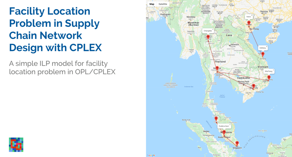
Oversimplified Case Study: Begpacker Inc.
The real world supply chain can be very complex. Consider the problem Begpacker Inc faced in the beginning: How can the CEO minimize his transportation cost while providing high service by meeting the customers’ demand?
| N | City | Demand (units) |
|---|---|---|
| 0 | Kuala Lumpur, MY | 187,000 |
| 1 | George Town, MY | 35,000 |
| 2 | Raffles Avenue, SG | 190,000 |
| 3 | Bangkok, TH | 172,300 |
| 4 | Chiang Mai, TH | 57,200 |
| 5 | Ho Chi Minh City, VN | 145,000 |
| 6 | Nha Trang, VN | 30,600 |
| 7 | Da Nang, VN | 61,000 |
| 8 | Hanoi, VN | 123,000 |
It is the most basic facility location problem. We are given a set of customer locations, deciding the number and locations of facilities (here plant-attached warehouse), so that the shipment costs can be minimized subject to meeting all customer demands.
Model Formulation
The Facility Location Problem can be formulated as an integer linear programming (ILP) model [1].
\begin{aligned}
\min \sum_i \sum_j c_{ij} \times d_{j} \times S_{ij} \quad & (1) \\
\end{aligned}
subject to
\begin{aligned}
\sum_i S_{ij} = 1 \quad \forall j \quad & (2) \\
\sum_i O_{ij} = m \quad \forall j \quad & (3) \\
S_{ij} \leq O_j \quad \forall i,j \quad & (4) \\
\end{aligned}
with decision variables
\begin{aligned}
& O_{i} = \begin{cases} 1  & \text{the facility at candidate site i} \in I\ \text{is opened} \\ 0 & \text{otherwise} \end{cases} \\
& S_{ij} = \begin{cases} 1  & \mathrm{shipping\ between\ candidate\ site\ i\ and\ demand\ site\ j} \\ 0 & \text{otherwise} \end{cases} \\
\end{aligned}
and other important parameters, as explained below:
c is the distance between facilities, also equivalent to cost, assuming the distance is linear to cost.
d is the demand in a city.
m is the total maximum number of facilities to be opened.
Since the candidate sites are same with the demand sites, so I = J.
Constraint (2) is a single sourcing contraint, stating each demand site is only served by one facility, while (3) requires the number of open facilities to be exactly m. Equation (4) is an indicator cosntraint requing the facility i to be open in order to ship from it to any demand site. The objective (1) is to minimize the total shipping cost, in our example just the number of units times the cost per unit.
Because there are no upper limit on the capacity of the production sites, any demand site will always be sourced from the production site with the cheapest transportation cost \forall j\ S_{ij} = \text{argmin}\ \lbrace c_{ij} \rbrace. The only reason why this model is a ILP is because of constraint (3).
Model
/*********************************************
 * OPL 12.10.0.0 Model
 * Author: diegoolivierfernandezpons
 * Creation Date: Oct 25, 2020 at 9:00:00 AM
 *********************************************/

int n = ...; // Number of cities
int m = ...; // Maximum number of facilities to be opened

range r = 0 .. n - 1;

int demand[r] = ...; // Demand
int cost[r][r] = ...; // Cost

dvar boolean Open[r]; // Open a facility at i
dvar boolean Ship[r][r]; // Ship from i to j

minimize sum (i,j in r) cost[i][j] * demand[j] * Ship[i][j];

constraints {

    // each demand site is shipped by only one facility
    forall (j in r) sum (i in r) Ship[i][j] == 1;

    // Total facilities opened limitation
    forall (j in r) sum (i in r) Open[i] == m;

    // Ship only if the facility is opened
    forall (i, j in r) Ship[i][j] <= Open[i];
}
Data
n = 9;
m = 3;
demand = [187000, 35000, 190000, 172300, 57200, 145000, 30600, 61000, 123000];
cost = [
[0,354,361,1490,2171,2346,2734,2603,2817]
[353,0,722,1170,1852,2026,2414,2283,2497]
[366,723,0,1859,2540,2715,3103,2972,3186]
[1490,1172,1859,0,686,862,1251,1118,1332]
[2185,1867,2554,700,0,1476,1827,1374,1396]
[2342,2024,2712,867,1471,0,433,960,1720]
[2731,2413,3101,1256,1819,434,0,529,1288]
[2597,2279,2967,1117,1384,962,529,0,769]
[2819,2501,3189,1339,1392,1724,1291,770,0]
];
Result
// solution (optimal) with objective 330459800
// Quality Incumbent solution:
// MILP objective                                 3.3045980000e+08
// MILP solution norm |x| (Total, Max)            1.20000e+01  1.00000e+00
// MILP solution error (Ax=b) (Total, Max)        0.00000e+00  0.00000e+00
// MILP x bound error (Total, Max)                0.00000e+00  0.00000e+00
// MILP x integrality error (Total, Max)          0.00000e+00  0.00000e+00
// MILP slack bound error (Total, Max)            0.00000e+00  0.00000e+00
//

Ship = [[1
             1 1 0 0 0 0 0 0]
             [0 0 0 0 0 0 0 0 0]
             [0 0 0 0 0 0 0 0 0]
             [0 0 0 1 1 1 1 0 0]
             [0 0 0 0 0 0 0 0 0]
             [0 0 0 0 0 0 0 0 0]
             [0 0 0 0 0 0 0 0 0]
             [0 0 0 0 0 0 0 0 0]
             [0 0 0 0 0 0 0 1 1]];
Open = [1 0 0 1 0 0 0 0 1];
Comment
Opened Facilities
Open = [1 0 0 1 0 0 0 0 1];We should open the facilities at site 0, 3 and 8 which are KualaLumpur, Bangkok and Hanoi.
Shipment
Ship = [[1
             1 1 0 0 0 0 0 0]
             [0 0 0 0 0 0 0 0 0]
             [0 0 0 0 0 0 0 0 0]
             [0 0 0 1 1 1 1 0 0]
             [0 0 0 0 0 0 0 0 0]
             [0 0 0 0 0 0 0 0 0]
             [0 0 0 0 0 0 0 0 0]
             [0 0 0 0 0 0 0 0 0]
             [0 0 0 0 0 0 0 1 1]];
Given maximum 3 facilities, we should ship from:
- facility 0 to sites 0, 1 and 2
KualaLumpur to KualaLumpur, GeorgeTown and RafflesAvenue - facility 3 to sites 3, 4, 5 and 6
Bangkok to Bangkok, ChiangMai, HoChiMinhCity and NhaTrang - facility 8 to sites 7 and 8
Hanoi to DaNang and Hanoi
Interestingly, the demand of Nha Trang and Ho Chi Minh (Vietnam) will be fulfilled by Bangkok (Thailand). We did not consider the cross boarder cost for this case study.
This case study seems to be too simplistic, i.e. it is only minimizing the weighted distance. However, this simple model can solve many supply chain network problems. Distance and transportation costs are highly correlated, i.e. the farther you have to go, the more expensive. This is a good approximation for minimizing the transportation costs. By having facilities as close to the customers as possible, indirectly providing better service levels.
If you’re interested to learn more how to model your real world supply chain and get great benefits from that, feel free to talk to us.
References
[1] Daskin, Mark S., Lawrence V. Snyder, and Rosemary T. Berger. 2005. “Facility Location in Supply Chain Design,” 39–65. https://www.lehigh.edu/~lvs2/Papers/facil-loc-sc.pdf