We were invited to give a talk about mathematical modeling of optimization problems to 4th year physics students. This material is based on that talk, and therefore intended to beginners with little knowledge about optimization, but a background in science.
Mathematical modeling in physics
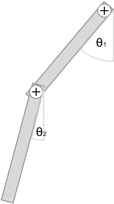
The inclined plane
A typical high-school physics exercise is the inclined plane
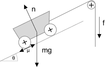
Students are expected to deduce the relation f = mg \sin \theta, sometimes with the friction \mu and from the Newton principle F = ma write the kinematic equations x = \dots by double integration (acceleration -> speed -> position)
The double pendulum
A typical classical mechanics exercise in university is the double pendulum.
The double pendulum is the first example where the kinematic equations cannot be written just by analyzing the figure.
The way to proceed is to write the Lagrangian of the system (the difference between potential and kinetic energy)
L = T - Vin this case we have
\begin{aligned}
& V = −2l \cos \theta_1 mg − l \cos \theta_2 mg\\
& T = \frac{1}{2} ml^2 \left ( \dot{\theta_1}^2 + \dot{\theta_2}^2 + 2 \dot{\theta_1} \dot{\theta_2} \cos (\theta_1 − \theta_2) \right )
\end{aligned}
The write the equilibrium condition (minimum of action)
\displaystyle\frac{d}{dt} \left ( \frac{\partial L}{\partial \dot{q}} \right) - \frac{\partial L}{\partial q} = 0And after some algebraic manipulations you get
\begin{aligned}
& 2l\ddot{\theta_1} + l\ddot{\theta_2} \cos (\theta_1 - \theta_2) + l\dot{\theta}^2_2 \sin (\theta_1 - \theta_2) + 2g\; \sin \theta_1 = 0 & \quad (1)\\
& l \ddot{\theta}_2 + l\ddot{\theta}_1 \cos (\theta_1 - \theta_2) + l \dot{\theta}^2_1 \sin (\theta_1 - \theta_2) + g\, \sin \theta_2 = 0 & \quad (2)
\end{aligned}
But unlike simpler examples, these equations cannot be manually solved (they don’t admit an analytic integral). The only way to proceed is to input them into a software that will solve them numerically.
One obtains a result that looks like this
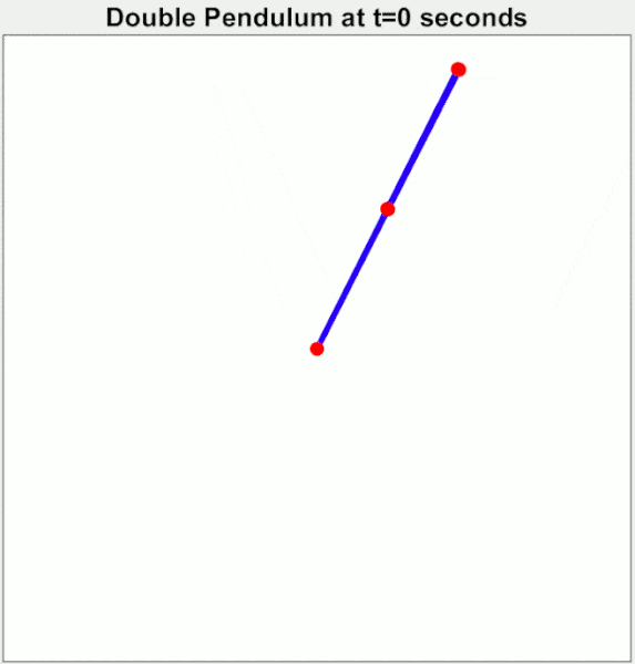
Image wikipedia
By the way, the double pendulum is also interesting because it is a very simple example of deterministic chaos (small changes in the initial position lead to important changes in the movement)
The modeling process in physics
For complex objects the process is
- Describe the object being studied (potential and kinetic energy)
- Add extra equations that convey its evolution
- Use a software to integrate numerically
Mathematical model in economy
Ricardo’s comparative advantage
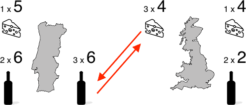
In 1817, economist David Ricardo wanted to show that it was beneficial for countries to engage in trade even with other countries that had cheaper production costs.
To show his point he devised the following example : Portugal and England can both produce cheese and wine. But labor is cheaper in Portugal therefore they always produce more with the same amount of people.
Imagine there are only 3 people in each country
- Portugal produces 1 x 5 cheese (5) and 2 x 6 bottles of wine (12)
- England produces 1 x 4 cheese (4) and 2 x 2 bottles of wine (4)
If instead each country specializes in the production they are the most efficient in, it gives
- Portugal 3 x 6 bottles of wine (18)
- England 3 x 4 cheese (12)
And we see the total production is higher than in the previous case. Therefore the countries can exchange and be better-off.
Modeling optimal production with linear programming
Today’s economists would model this problem with the following equations (called an integer linear program)
\begin{aligned}
\max \, 6 p_w + 5 p_c + 2 e_w + 4 e_c &\\
\\
p_w + p_c = 3 & \\
e_w + e_c = 3 & \\
\\
p_w, p_c, e_w, e_c \in \mathbb{N}
\end{aligned}
Obviously this model of international trade is extremely simplistic and fails to capture many important characteristics of international trade.
However the principle remains, economists use mathematical equations on a regular basis to quantify economic phenomena and investigate what is the optimal usage of resources
Optimal usage of resources
Linear programming was invented by the mathematician Leonid Kantorovich in 1939, for which he received the Nobel price in economy in 1975, shared with Tjalling Koopmans, for for their contributions to the theory of optimum allocation of resources.
George Dantzig published in 1947 the simplex algorithm that solves linear programs in a systematic way (Kantorovitch used to do it by hand). It was later extended to (mixed) integer programming, which is the tool that is used today.
Integer programming can be used to solve a large variety of optimal resource allocation problems
- manufacturing
- transportation
- time tables and schedules
- location of facilities
Modeling industrial problems
The discipline that solves (industrial) resource allocation problems / optimization problems is not clearly defined. It is sometimes
- computer science
- management science
- operations research
- applied mathematics
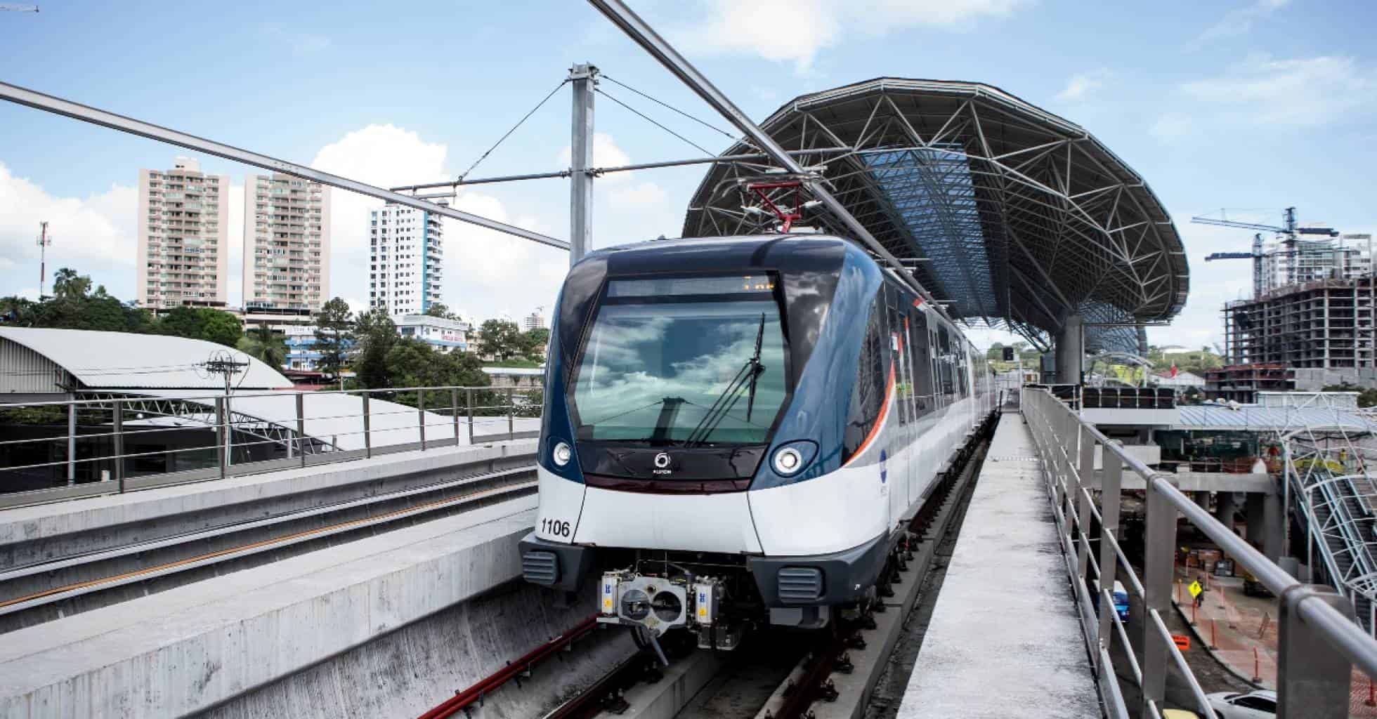
Let’s model a subway line to compute the minimum number of trains needed to transport all passengers.
Ignoring time
Consider a subway line with only one direction, 3 stations, a capacity of 20 for each subway and the following amount of people wanting to move from one point to another.
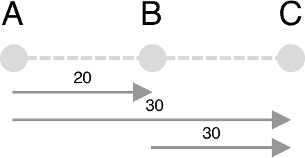
We will ignore the temporal dimension.
To compute the number of trains needed we just compute for each section of line the total ridership and divide it by the capacity
\begin{aligned}
  & \max \left ( \left \lceil \frac{20 + 30}{20} \right \rceil, \left \lceil  \frac{30 + 30}{20} \right \rceil \right )\\
  \leadsto \quad & \max \left ( \lceil 2.5 \rceil, \lceil 3 \rceil \right )\\
  \leadsto \quad & \max \left ( 3 ,  3 \right )\\
  \leadsto \quad & 3
\end{aligned}
Written as a symbolic formula
N = \max_{i} \left \lceil \displaystyle\frac{1}{\mathrm{capacity}} \sum_{o\, \leq\, i \wedge \, i + 1\, \leq\, d} \mathrm{traffic}^{od} \right \rceil This case was so simple that we were able to guess the formula from the problem.
Adding the time dimension
Once we add a time dimension to the problem, there are new aspects that need to be considered.
- people will start accumulating on station platforms
- the train moves from station station
- the train arrives with people from the previous station
- there is a minimum time between trains
Just guessing a formula is too complicated. The only viable approach is the same used for complex physics problems : describe the properties of the problem with equations and give the equations to a software to solve
For instance the accumulation of people on station platforms can be written
\forall i,\ \forall t,\ \mathrm{platform}^t_i = \mathrm{platform}^{t - 1}_i + \mathrm{arrived}^t_i - \mathrm{entered}^t_iIn plain words
The amount of people on the platform of station
iat timetis the number of people on the platformitimet - 1plus the people that arrived at the station at timet, minus the people that entered the subway that passed at timet
We will need a similar equation for each train to account for the number of people entering and exiting a train. But the train moves. In order to simplify the problem we will consider it takes 1 time unit for a train to move from one station to the next.
In other words the train leaving station i at time t is the same arriving at station i + 1 at time t + 1
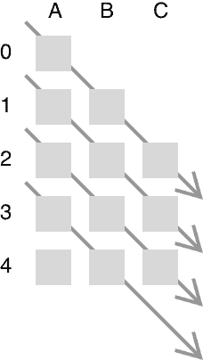
Then the accumulation of people in the train can be written
\forall i,\ \forall t,\ \mathrm{train}^t_i = \mathrm{train}^{t - 1}_{i - 1} + \mathrm{entered}^t_i - \mathrm{exited}^t_iWe finally need to add a variable to capture the fact that a train may or may not leave station A at time t.
\mathrm{leave}_t \in \lbrace 0, 1 \rbraceAnd the fact that if there is no train at time t on station i, then nobody can enter or exit the (non existing) train.
\begin{aligned}
& \forall i,\ \forall t,\
\mathrm{entered}^t_i \leq \mathrm{capacity} \times \mathrm{leave}_{t - i}\\
& \forall i,\ \forall t,\
\mathrm{exited}^t_i \leq \mathrm{capacity} \times \mathrm{leave}_{t - i}
\end{aligned}
Finally we add the capacity limit of each train
\forall i,\ \forall t,\ \mathrm{train}^t_i \leq \mathrm{capacity} \times \mathrm{leave}_{t - i} We also need to take care of all the index problems – the special case for each equation when some indexes make no sense like v^{t - 1} with t = 0
Putting it all together
The full set of equations becomes (we omit corner cases)
\begin{aligned}
& \min \sum_t \mathrm{leave}_t\\
\\
&\forall i,\ \forall t,\ \mathrm{train}^t_i \leq \mathrm{capacity} \times \mathrm{leave}_{t - i} & \quad (1)\\
&\forall i,\ \forall t,\ \mathrm{platform}^t_i = \mathrm{platform}^{t - 1}_i + \mathrm{arrived}^t_i - \mathrm{entered}^t_i & \quad (2)\\
& \forall i,\ \forall t,\ \mathrm{train}^t_i = \mathrm{train}^{t - 1}_{i - 1} + \mathrm{entered}^t_i - \mathrm{exited}^t_i & \quad (3)\\
& \forall i,\ \forall t,\
\mathrm{entered}^t_i \leq \mathrm{capacity} \times \mathrm{leave}_{t - i} & \quad (4)\\
& \forall i,\ \forall t,\
\mathrm{exited}^t_i \leq \mathrm{capacity} \times \mathrm{leave}_{t - i} & \quad (5)\\
\end{aligned}
And when you put everything into a computer, it doesn’t work !
The problem is there is no constraint saying "people should get into the first train that has room". With this model, people are free to stay for ever on the platform if they wish. And that’s actually what minimizes the number of trains : people getting to the platform and never entering in any train.
Adding delays
First we need to express the fact that people get off where they are supposed to. We will express that saying the total number of people entering and exiting has to be equal to the values in the traffic matrix
\begin{aligned}
& \forall i\ \sum_t \mathrm{entered}^i_t = \sum_t \mathrm{arriving}^i_t\\
& \forall i\ \sum_t \mathrm{exited}^i_t = \sum_t \mathrm{leaving}^i_t\\
\end{aligned}
Then we need quantify the time spent between the arrival to the platform i and the exit at station j. This would be obvious if we had individual data but here we have only aggregate numbers.
It may help to look at an example. The first line is the people in the platform, the second line those entering the trains
10 10  5  0  0  0
 5  5  5  5  5  0
The delays per passenger look like this
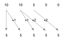
Let’s count 1 unit of delay per person per time period. Then the total delay in the figure is 30 = 1 5 + 1 5 + 2 5 + 2 5. We now need to perform the same computation without using the individual information (which passenger enter in which train).
We can achieve that by computing the cumulative of each array
10 10  5  0  0  0
10 20 25 25 25 25

 5  5  5  5  5  0
 5 10 15 20 25 25
And then taking the difference
10 20 25 25 25 25
 5 10 15 20 25 25
------------------
 5 10 10  5  0  0
And the sum gives 30
Playing with a couple of other examples one ends convincing oneself that this is not just a coincidence.
The formula is
delay = \sum_i \sum^i_{j = 1} \mathrm{arrival}_j - \mathrm{departure}_jNow that we have a delay formula we can change the objective of the linear program for a lexicographic objective (delay, quantity). The optimization software will first try to minimize the total delay, and then minimize the number of trains used.
The result looks like this
leave =      [1  1  1  1  1  0 0 0 0 0];
train =    [[20 20 20 17  5  0 0 0 0 0]
             [0 20 20 20 20  5 0 0 0 0]
             [0  0  0  0  0  0 0 0 0 0]];
enter =    [[20 20 20 17  5  0 0 0 0 0]
             [0 20 20  0  3  0 0 0 0 0]
             [0  0  0  0  0  0 0 0 0 0]];
exit =      [[0  0  0  0  0  0 0 0 0 0]
             [0 20 20  0  0  0 0 0 0 0]
             [0  0 20 20 20 20 5 0 0 0]];
platform = [[11 10 22  5  0  0 0 0 0 0]
            [19  7  3  3  0  0 0 0 0 0]
             [0  0  0  0  0  0 0 0 0 0]];
The OPL code
The most practical language (in our opinion) to write optimization models is OPL as it stays quite close to the mathematical notation.
OPL programs are solved with the optimization engine IBM ILOG OPL Cplex Studio.
/*********************************************
 * OPL 12.10.0.0 Model
 * Author: diegoolivierfernandezpons
 * Creation Date: Dec 3, 2020 at 9:15:12 PM
 *********************************************/

 //////////
 // Data //
 //////////

 int capacity = 20;
 int nb_stations = 3;
 int nb_time_points = 10;

 range time = 0 .. nb_time_points - 1;
 range stations = 0 .. nb_stations - 1;

 // Random traffic matrix
 int traffic [i in stations][j in stations][t in time] = (i < j) * rand(capacity) * (t < nb_time_points div 3);
 int arriving [j in stations][t in time] = sum (i in stations) traffic[i][j][t];
 int leaving [i in stations][t in time] = sum (j in stations) traffic[i][j][t];

 ///////////
 // Model //
 ///////////

 dvar boolean leave [time];
 dvar int+ platform [stations][time];
 dvar int+ train [stations][time];
 dvar int+ enter [stations][time];
 dvar int+ exit  [stations][time];

 dexpr int delayed [j in stations][t in time] = sum (s in time : s <= t) (arriving[j][s] - exit[j][s]);

 dexpr int delay = sum (i in stations, t in time) delayed[i][t];
 dexpr int usage = sum (t in time) leave[t];

 minimize staticLex (delay, usage);

 constraints {

    // Train capacity
    forall (t in time, i in stations : t - i in time) train[i][t] <= capacity * leave[t - i];
    forall (t in time, i in stations : t < i) train[i][t] == 0;

     // People inside train
    forall (i in stations, t in time : i - 1 in stations && t - 1 in time) train[i][t] == train[i - 1][t - 1] + enter[i][t] - exit[i][t];
    forall (i in stations : i - 1 in stations) train[i][0] == enter[i][0] - exit[i][0];
    forall (t in time : t - 1 in time) train[0][t] == enter[0][t] - exit[0][t];

    // People waiting in platform
    forall (i in stations, t in time : t - 1 in time)  platform[i][t] == platform[i][t - 1] - enter[i][t] + leaving[i][t];
    forall (i in stations) platform[i][0] == - enter[i][0] + leaving[i][0];

    // People can enter or exit only if train is present
    forall (i in stations, t in time : t - i in time) enter[i][t] <= capacity * leave[t - i];
    forall (i in stations, t in time : t - i in time) exit[i][t] <= capacity * leave[t - i];
    forall (i in stations, t in time : t < i) enter[i][t] == 0;
    forall (i in stations, t in time : t < i) exit[i][t] == 0;

     // People exit in the right place
    forall (i in stations) sum (t in time) exit[i][t] == sum (t in time) arriving[i][t];
    forall (i in stations) sum (t in time) enter[i][t] == sum (t in time) leaving[i][t];

 }