Line Balancing Problem

In a previous post we introduced various models for the mixed-model sequencing problem (MMSP), which consists in sequencing models to be produced in an assembly line that can produce different types of models.

Assembly line of Lotus. Image Wikimedia

In this post we are going to review models for the assembly line balancing problem which is the problem of assigning tasks to stations along the assembly line.

Tasks and precedences

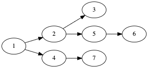
The first requirement to create an assembly line is to divide the work to be done into tasks and create a precedence diagram for the tasks.

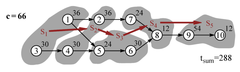
Precedence diagram from the very complete website on ALBP https://assembly-line-balancing.de (copyright Armin Scholl)

Tasks can be modeled at various granularity levels. The smaller the tasks, the more complex and computationally hard the optimization problem, but also the more efficient the assembly line.

Balanced bin-packing with precedences

The different tasks now need to be put into bins that correspond each to one station along the assembly line.

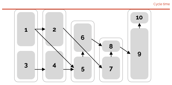
Bin-packing with precedences corresponding to the ALBP precedence graph

The tasks correspond to the operations the people in that station will have to complete on the product being built. The weight of each item in the bin-packing problem corresponds to the duration of the task. Thereafter, the product being built will spend $T_s = \sum_i t^i x^i_s$ time on station $s$ where $t^i$ is the team of the task $i$ and $x^i_s$ a decision variable that defines whether task $i$ has been assigned to station $s$ .

The cycle time of the assembly line is the average time spent in each station. But because we are not sequencing the units yet, we can consider that the cycle time will be limited by the longest time spent in any station.

An assembly line is said to be balanced when the time in each station is more or less the same.

Optimizing Cycle time and number of stations

The simple assembly line balancing problem has to important parameters

the cycle time c
the number of stations m

From there, there are various variants that are possible. For all variants, a precedence graph of tasks is given.

SALBP-1: Given the cycle time c, minimize the number of stations m
SALBP-2: Given the number of stations m, minimize the cycle time c.
SALBP-E: Given feasible ranges for m and c, maximize the line efficiency, which is equivalent to minimize the line capacity m * c.

CP models for the simple assembly-line balancing problem (SALBP-E)

We will fist use IBM ILOG CP Optimizer to solve the line capacity maximization problem (SALBP-E) as the problem is general quadratic (its objective is the product of two integer values)

The data

SALBP benchmark instances contain the following data

a precedence graph
an interval of acceptable number of stations

/*********************************************
 * OPL 12.10.0.0 Model
 * Author: diegoolivierfernandezpons
 * Creation Date: Aug 18, 2020 at 7:45:36 PM
 *********************************************/

 using CP;

 // Data

 tuple precedence_T { int pred; int succ; }

 int nb_tasks = ...;
 int min_stations = ...;
 int max_stations = ...;

 range stations = 1 .. max_stations;
 range tasks = 1 .. nb_tasks;

 {precedence_T} precedences = ...;
 int duration [p in tasks] = ...;

The using CP line instructs OPL to use CP Optimizer as solver

The pack constraint

CP Optimizer includes a constraint specially to solve the bin-packing problem and its variants. Consider a bin-packing problem with n items to be packed into m bins, then the constraint pack (load, where, weight, m) works as follows

weight is an array of n integers that correspond to the weights of the items
where is an array of n decision variables that correspond to the location (the bin number) of the items
load is an array of m decision variables that corresponds to the sum of the weights of the items packed in each bin
m is a decision variable that corresponds to the number of bins used

The equivalent MILP formulation would be

 $\begin{aligned} \forall i \in items \quad \text{where}^i = \sum_b b * \text{where\_binary}^i_b & \quad (1)\\ \forall b \in bins \quad \text{load}_b = \sum_i \text{weight}^i * \text{where\_binary}^i_b & \quad (2)\\ \forall b \in bins \quad \text{where\_binary}^i_b \leq \text{used}_b & \quad (3)\\ \forall b \in bins \quad \text{used}_b \geq \text{used}_{b + 1} & \quad (4)\\ m = \sum_b \text{used}_b & \quad (5)\\ \forall i \in tasks \quad \sum_b \text{where\_binary}^i_b = 1 & \quad(6)\\ \\ \text{where\_binary}^i_b \in \lbrace 0, 1 \rbrace \quad \quad &\\ \text{used}_b \in \lbrace 0, 1 \rbrace \quad \quad &\\ \text{where}^i \in \mathbb{N} \quad \quad &\\ \text{load}_b \in \mathbb{N} \quad \quad &\\ m \in \mathbb{N} \quad \quad &\\ \end{aligned}$

Notice how CP Optimizer prefers working directly with integer variables. It is always possible to define the binary variables if needed but CP Optimizer’s API won’t force that by default.

Minimization of idleness

The results in the benchmark we will use are reported in terms of total idle time which is $m * c - \sum_i t^i$ . As the sum of the durations of the tasks is a constant, this doesn’t change the problem

We can now continue the model

 int t_sum = sum (p in tasks) duration[p];

 // Model

 dvar int station [p in tasks] in stations;
 dvar int time [stations] in 0 .. t_sum;
 dvar int m in min_stations .. max_stations;

 dexpr int c = max (s in stations) time[s];
 dexpr int idle = m * c - t_sum;

 minimize idle;

 constraints { 

    // Packing constraint (1)
    pack (time, station, duration, m);

    // Precedences (2)
    forall (<p, q> in precedences) station[p] <= station[q];
}

Precedences

For the precedences we simply write that if <p,q> appreas in the precedences, then the location of p is smaller than the location of q

Redundant constraints based on item size

Redundant constraints are equations that are not required for the problem to be correct but improve its resolution speed as they allow the solver to make better deductions.

Precedence-energy

While the previous model is enough to solve the SALBP, adding redundant constraints may make the model perform better. These are constraints that are optional but help the engine make better deductions.

The precedence-energy deduction rule ("raisonnement énergétique" in French) was introduced by Pierre Lopez in his PhD thesis "Approche énergétique pour l’ordonnancement de tâches sous contraintes de temps et de ressources" (1991) [1]. Subsequent publications (in English) are also available online.

If an item were to be packed in bin $b$ there should be enough capacity for all the predecesors of this item in the bins preceding $b$ , and symetrically in the bins following $b$

 $\forall q \in items \quad \left (\text{where}^q = b \right) \Rightarrow \left ( \sum_1^{b} \text{load}_k \geq \sum_{p \prec q} \text{weight}^p \right )$

Which can be upper-bounded by

 $\forall q \in items \quad \sum_{p \prec q} \text{weight}^p \leq \text{where}^q * \max_k \text{load}^k$

We have chosen this approximation because the max of the loads in our problem is exactly the cycle time.

We hence add to the data section of the OPL model the necessary to compute the longest path between tasks (the transitive closure of the precedence graph) and the list of predecessors and successors of each task.

// Longest path computation
int d [p in tasks][q in tasks] = 0;
execute {
    for (var k in precedences) d[k.pred][k.succ] = 1;
    for (var k in tasks)
        for (var i in tasks) if (d[i][k] > 0)
            for (var j in tasks) if (d[k][j] > 0) {
                var c = d[i][k] + d[k][j];
                if (d[i][j] < c) d[i][j] = c;
            }    
 } 

// List of Predecessors and successors
{int} pred [q in tasks] = { p | p in tasks : d[p][q] > 0 } union { q };
{int} succ [p in tasks] = { q | q in tasks : d[p][q] > 0 } union { p };

// Total duration of predecessors / successors
int sumPred [q in tasks] = sum (p in pred[q]) duration[p];
int sumSucc [p in tasks] = sum (q in succ[p]) duration[q];

And to the constraint section the lines

// Precedence-energy approx (3)
forall (q in tasks) sumPred[q] <= c * station[q];
forall (p in tasks) sumSucc[p] <= c * (m - station[p] + 1);

We can also write the traditional precedence-energy

dexpr int sumBefore [s in stations] = sum (k in stations : k <= s) time[k];
dexpr int sumAfter [s in stations] = sum (k in stations : k >= s) time[k];

// Precedence-energy (4)
forall (q in tasks) sumPred[q] <= sumBefore [station[q]];
forall (p in tasks) sumSucc[p] <= sumAfter [station[p]];

Earliest start time / latest completion time

Let’s rewrite the precedence-energy equations in a different way

// Precedence-energy (3')
forall (q in tasks) station[q] >= sumPred[q] / c;
forall (p in tasks) station[p] <= (m + 1) - sumSucc[p] / c;

The precedence-energy constrant is actually computing earliest start time / latest completion time bounds for the tasks. In a traditional bin-packing problem, the size $c$ of the bins would be fixed and the equations would be pure constants LB <= station[p] <= UB. In this problem however the bounds keep improving as the engine finds better bounds for the cycle time $c$ .

Minimal distance between tasks

In the same way we applied precedence-energy to compute minimal distances between tasks and the first and last bins, we can apply it to compute minimal distances between tasks

To do so, we just compute the total duration of tasks between any pair (p, q) of tasks

{int} mid [p in tasks][q in tasks] = succ[p] inter pred[q];
int sumMid [p in tasks][q in tasks] = sum (k in mid[p][q]) duration[k];

And we apply the same technique, noticing however that if $p \prec q$ and they are assigned to the same bin / station, then $0 < \frac{t_p + t_q}{c} < 1$ hence the -1 term in the equation.

// Distance between tasks (5)
forall (p, q in tasks : card (mid[p][q]) > 0)
    station[p] + sumMid[p][q] / c - 1 <= station[q];

Conflict based distance between tasks

When the size of the bin is small with respect to the items, items cannot be packed together which creates incompatibilities

In MIP these incompatibilities would be collected by the clique graph. In a bin-packing problem with precedenced we are going to try to transform them into precedences instead.

Therefore we introduce the following constraint

// Conflicts (6)
forall (p, q in tasks : p != q && q in succ[p])
    station[p] + (duration[p] + duration[q] > c) <= station[q];

Surrogate knapsack constraint

Surrogate knapsack constraints are typical in bin-packing problems. They are a weak version of the energetic reasoning which says

There shall be enough capacity for all subsets of items

Here we apply it to the set of all items in a form that involves the cycle time $c$ and one that involves the bin loads time[s]

// Surrogate knapsack (7)
m * c >= t_sum;

The term surrogate knapsack comes from the fact they are the sum of all the knapsack constraints in a MIP formulation

 $\begin{aligned} & \forall b \in bins\quad \sum_i w^i * x^i_b \leq C\\ \Rightarrow \quad & \sum_b \sum_i w^i * x_b^i \leq \sum_b C\\ \leadsto \quad & \sum_i w^i \leq \ \mid bins \mid *\ C\\ \end{aligned}$

Making redundant constraints dynamic

Transitivity of the precedence

Notice that in all the previous equations, while $c$ is a variable that is adjusted by the engine as the resolution of the problem progresses, the durations of the predecessors / successors sumPred and sumSucc are constants computed at the root of the solution process.

Concretely what the precedence-energy constraint means is that when solving the JACKSON instance (precedence graph below), if the engine decides to schedule 7 before 8, in other words add the precedence $7 \prec 8$ then there needs to be "enough room" for all the old { 1 2 6 } and new { 1 3 4 5 7 } predecessors of 8

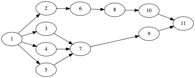
Precedence graph for JACKSON

With a static implementation of sumPred, the new predecessors won't be taken into account. A dynamic implementation can be obtained by introducing the following expressions

dexpr int before [p in tasks][q in tasks] = station[p] <= station[q];

dexpr int sumPred [q in tasks] = sum (p in tasks) before[p][q] * duration[p];
dexpr int sumSucc [p in tasks] = sum (q in tasks) before[p][q] * duration[q];

Now precedence-energy can be written as an equality

// Precedence-energy (4')
forall (q in tasks) sumPred[q] == sumBefore [station[q]];
forall (p in tasks) sumSucc[p] == sumAfter [station[p]];

We can also replace the precedence constraint with

// Precedences (2')
forall (p in tasks, q in succ[p]) before[p][q] == 1;

Dynamic distance between tasks

In the distance constraint there are various elements that are computed at the root node and never updated as the solver makes progress in the tree

sumMid : the total duration of tasks between two tasks
dist : the distance between tasks

dexpr int dist [p in tasks][q in tasks] = station[q] - station[p];

// Distance between tasks (5')
forall (p, q in tasks : p != q && q in succ[p])
    dist[p][q] >= sumMid[p][q] / c - 1;

// Conflicts (6')
forall (p, q in tasks : p != q && q in succ[p])
    dist[p][q] >= (duration[p] + duration[q] > c);

We can also attempt to propagate the changes in the distances with Bellman-like shortest path equations

dvar int dist [tasks][tasks] in - max_stations .. max_stations;

// Propagation of distances (8)
forall (p, q in tasks)
    dist[p][q] == (station[q] - station[p]);

forall (p in tasks, r in succ[p] : r != p, q in succ[r] : q != r && q != p) 
    dist[p][q] >= dist[p][r] + dist[r][q];

Redundant constraints based on cardinality

In a subsequent blog post we will discuss how to use cardinality argument in bin-packing [2]. Otherwise it would make this blog post too long. We will however show some examples of cardinality constraints based on precedence.

Tasks without predecessors / successors

We defined $m$ as a variable in min_stations .. max_stations. There is nothing in the present formulation that prevents $m$ to be very large say 10, but there are no items between 5 and 10. Instead we can define $m$ to be the max of the tasks without any successor.

We can add that property in the definition of m

dexpr int m = max (p in tasks : card(succ[p] == 1) station[p]);

// Bounds on m (9)
min_stations <= m <= max_stations;

Or we can leave $m$ defined as a decision variable and add the property as a constraint

dvar int m in min_stations .. max_stations;

// Maximum of tasks without successor (9')
max (p in tasks: card(succ[p]) == 1) station[p] == m;

We can also write the symmetric constraint

// Minimum of tasks without predecessor (10)
min (p in tasks: card(pred[p]) == 1) station[p] == 1;

Precedence with cardinality

Now consider the Mertens precedence graph with $m \in [5 .. 5]$ .

Precedence graph of MERTENS instances

CPO tries to push the node 6 to station 1 without noticing that if it does that, there won't be enough remaining nodes after 6 (that is 4, 3, 7) to have one per bin.

To prevent this problem we can add the constraint

forall (p in tasks) station[p] >= m - sum (q in tasks) after[q][p];

Where after[p][q] is 1 - before[p][q] and the constraint can be rewritten

dexpr int cardPred[p in tasks] = sum (q in tasks) before[q][p]
dexpr int cardSucc[p in tasks] = sum (p in tasks) before[q][p]

// At least on item per bin (11)
forall (p in tasks) station[p] >= m + 1 - cardSucc[p];
forall (p in tasks) station[p] <= cardPred[p];

We can also introduce

dexpr int number[s in stations] = sum (p in tasks) (station[p] == s);

dexpr int cardBefore [s in stations] = sum (k in stations : k <= s) number[k];
dexpr int cardAfter [s in stations] = sum (k in stations : k >= s) number[k];

// Precedence-cardinality (12)
forall (q in tasks) cardPred[q] == cardBefore [station[q]];
forall (p in tasks) cardSucc[p] == cardAfter [station[p]];

While these are the cardinality equivalent of precedence-energy, they are likely not to be very useful as $c$ is large with respect to $t^p$ .

Other improvements

Bounding of the cycle time

Having an upper bound on $c$ allows better deductions from the beginning as many constraints have $c$ in the denominator like

forall (q in tasks) station[q] >= sumPred[q] / c;

The minimum value for station[q] is computed by dividing the minimum value of sumPred[q] with the maximum value of $c$ .

According to [3] citing [7] a valid upperbound for $c$ is given by

 $\overline{c} = \max \left \lbrace \left ( \max_p t^p \right ), 2 * \left ( \sum_p t^p \right ) / \underline{m} \right \rbrace$

While we haven't been able to check reference [7] as it is not available online, the different solvers find a large number of solutions with $c \lt \overline{c}$ which provides ample experimental support.

Variables versus expressions

Some (mathematical) variables can be defined as decision variables or as decision expressions. Typical examples include c, m, etc.

Depending on the choice made, the engine may or may not branch on them, which may or may not be beneficial. There are also some subtle differences in the propagation (deduction power).

Therefore all variants need to be tested.

MIP models for the simple assembly-line balancing problem (SALBP-E)

Our basic MIP mode is slightly different than [3] as we prefere writing constraints with equalities first, and checking later if removing variables improves the running times.

 $\begin{aligned} \min \sum_s i_s \quad \quad \\ \forall s \in \text{stations} \quad \sum_p t^p * x^p_s + i_s + f_s = c & \quad (1)\\ \forall s \in \text{stations} \quad f_s \leq \overline{c} * (1 - y_s) & \quad (2)\\ \forall s \in \text{stations} \mid s \leq \underline{m} \quad y_s = 1 & \quad (3)\\ \\ \forall p \in \text{tasks} \quad \sum_s x^p_s = 1 & \quad (4)\\ \forall s \in \text{stations},\ p \in \text{tasks} \quad x^p_s \leq y_s & \quad (5)\\ \forall s \in \text{stations} \quad y_s \leq \sum_i x^i_s & \quad (6)\\ \forall s \in \text{stations} \quad y_s \geq y_{s + 1} & \quad (7)\\ \forall\ p \prec q \in \text{tasks} \quad \sum_s s * x^p_s \leq \sum_s s * x^q_s & \quad (8)\\ x^i_s \in \lbrace 0, 1 \rbrace & \\ y_s \in \lbrace 0, 1 \rbrace & \\ c \in \mathbb{N} &\\ i_s \in \mathbb{R}^+ & \\ f_s \in \mathbb{R}^+ & \\ \end{aligned}$

The knapsack equation with explicit slack variables ("wasted space") is typically written $\sum_k a_k x_k + s = C * y$ where $C$ is a constant. In our case it is a variable, hence we cannot multiply it by $y$ . Instead we add a filler variable $f_s$ that will "absorb" all the value of $c$ when the bin is not used (1). To do so we constrain $f_s$ to zero when $y_s$ is one (2), and
(3) fixes to "used" all the bins before the minimum number of bins

Equation (4) says tasks need to be packed in exactly one bin. (5) and (6) link the content of each bin $x^p_s$ and the usage indicator $y_s$ . While (7) ensures bins are used from left to right. Equation (8) establishes the precedence between tasks.

Other linearizations

Esmaeilbeigi et al. [3] chose a slightly different way of coping with the bins that are not used

 $\begin{aligned} \forall s \in \text{stations}\ |\ s \leq \underline{m} \quad \sum_p t^p * x^p_s + i_s = c & \quad (1a)\\ \forall s \in \text{stations}\ |\ s \gt \underline{m} \quad \sum_p t^p * x^p_s \leq c & \quad (1b)\\ \forall s \in \text{stations}\ |\ s \gt \underline{m} \quad \sum_p t^p * x^p_s + i_s \geq c - \overline{c} * (1 - y_s) & \quad (1c)\\ \forall s \in \text{stations}\ |\ s \gt \underline{m} \quad \sum_p t^p * x^p_s + i_s \leq \overline{c} * y_s & \quad (2)\\ \end{aligned}$

This lineairzation is somehow similar - our linearization just replaces $\overline{c} * (1 - y_s)$ with a continuous variable $f_s$ and $f_s \leq \overline{c} * (1 - y_s)$ .

The main difference is that our linearization allows the surrogate knapsack constraints to be written in an equality for $\overline{m} * c = \sum_p t^p + \sum_s i_s + \sum_s f_s$ . The authors of [3] don't add a surrogate constraint, but if they had, it would have to be written $\overline{m} * c \geq \sum_p t^p + \sum_s i_s$

Corominas et al. [6] suggest a linearization of the $m * c$ objective where there is one binary variable for every value of $m$ between $\underline{m}$ and $\overline{m}$ . We will consider this linearization in a subsequent benchmark.

Redundant constraints

Some of the redundant constraints used in the CPO models can be used in the MIP model. The main difference being that the CPO model could cope with non-linear constraints (general integer products) while MIP engines can only under certain conditions.

Because of that, in some cases we were only able to try static constraints in the sense they are computed at the root node using bounds like $\overline{c}$ .

The constraints are

Root-node precedence-energy (9 - 10)
Surrogate knapsack (11)
Root-node distance (12 - 13)
Conflicts using indicator constraints (14)

 $\begin{aligned} \forall q \in \text{tasks},\ s \in \text{stations} \quad \left (\sum_{p \prec q} t^q \right) * x^q_s + \sum_{k \leq s} (i_k + f_k) \leq s * c & \quad (9)\\ \forall p \in \text{tasks},\ s \in \text{stations} \quad \left (\sum_{p \prec q} t^q \right) * x^p_s + \sum_{k \geq s} (i_k + f_k) \leq (\overline{m} - s + 1) * c & \quad (10)\\ \overline{m} * c = \sum_s i_s + f_s + \sum_p t_p & \quad (11)\\ \forall p \in \text{tasks} \quad z^p = \sum_s s* x^p_s & \quad (12)\\ \forall p \prec q \in \text{tasks} \quad z^q - z^p \geq \text{sumMid}^{pq} / \overline{c} - 1 & \quad (13)\\ \forall p, q \in \text{tasks}, \forall s \in \text{stations} \quad (t^p + t^q \geq c + 1) \Rightarrow (x^p_s + x^q_s \leq 1) & \quad (14)\\ z^p \in \mathbb{N} & \\ \end{aligned}$

We don't expect conflicts using indicator constraints to be very useful due to the internal linearization Cplex needs to do to handle the implication. Notice how this constraint would be simply handled by the clique graph if $c$ was a constant.

We expect root-node constraints to have a some impact on smaller instances but almost nothing on large instances - they are basically a form of pre-processing.

We expect the surrogate knapsack constraint to have the most effect.

Implied integer variables

A variable is said to be implied integer when it will take an integer value even if declared continuous due to other integer values. This happens very often in equality constraints like

 $\begin{aligned} \sum_k a_k \times x_k + s = c \times y \\ x_k, y \in \lbrace 0, 1 \rbrace \quad a_k, c \in \mathbb{Z} & \\ \\ \sum_k k \times x_k = s & \\ x_k \in \lbrace 0, 1 \rbrace &\\ \end{aligned}$

Implied integers can be declared integer

The MIP engine may branch on them and will attempt to generate cuts involving them
The MIP heuristics will suffer from the extra variables

Implied integers can be declared continuous

The MIP problem will have less variables to branch on - the problem is smaller

Our model has many implied integer variables like $z^p$ (position of the items) or groups of variables where as soon as one is declared integer the other ones become implied like $c$ , $i_s$ (wasted space per bin) and $f_s$ (filler).

MIP model in OPL

The most complete model is the following.

/*********************************************
 * OPL 12.10.0.0 Model
 * Author: diegoolivierfernandezpons
 * Creation Date: Aug 22, 2020 at 7:38:25 PM
 *********************************************/

 // Data

 tuple precedence_T { int pred; int succ; }

 int nb_tasks = ...;
 int min_stations = ...;
 int max_stations = ...;

 range stations = 1 .. max_stations;
 range tasks = 1 .. nb_tasks;

 {precedence_T} precedences = ...;
 int duration [p in tasks] = ...;

 int t_sum = sum (p in tasks) duration[p];
 int t_max = max (p in tasks) duration[p];

 int ub_c = maxl (t_max, ftoi(floor(2 * (t_sum - 1) / min_stations)));

 int d [p in tasks][q in tasks] = 0;
 execute {
    for (var k in precedences) d[k.pred][k.succ] = 1;
    for (var k in tasks)
        for (var i in tasks) if (d[i][k] > 0)
            for (var j in tasks) if (d[k][j] > 0) {
                var c = d[i][k] + d[k][j];
                if (d[i][j] < c) d[i][j] = c;
            }    
 } 

 {int} pred [q in tasks] = { p | p in tasks : d[p][q] > 0 } union { q };
 {int} succ [p in tasks] = { q | q in tasks : d[p][q] > 0 } union { p };
 {int} mid [p in tasks][q in tasks] = succ[p] inter pred[q];

 int sumPred [q in tasks] = sum (p in pred[q]) duration[p];
 int sumSucc [p in tasks] = sum (q in succ[p]) duration[q];
 int sumMid [p in tasks][q in tasks] = sum (k in mid[p][q]) duration[k];

 // Model

 dvar boolean x [tasks][stations] in 0 .. 1;
 dvar boolean y [stations];

 dvar int c in 1 .. t_sum;
 dvar int station [tasks] in stations;

 dvar float id [stations] in 0 .. t_sum;
 dvar float fill [stations] in 0 .. t_sum;

 minimize sum (s in stations) id[s];

 constraints {

    // Capacity
    forall (s in stations) sum (i in tasks) duration[i] * x[i][s] + id[s] + fill[s] == c ;

    // Filler only for unused bins
    forall (s in stations) fill[s] <= ub_c * (1 - y[s]);

    // Each item goes into one bin
    forall (i in tasks) sum (s in stations) x[i][s] == 1;

    // A bin is used if it has at least one item
    forall (s in stations, i in tasks) x[i][s] <= y[s];
    forall (s in stations) y[s] <= sum (i in tasks) x[i][s];

    // Minimum number of used bins
    forall (s in stations : s <= min_stations) y[s] == 1; 

    // Bins are used from left to right 
    forall (s in stations : s + 1 in stations) y[s] >= y[s + 1];

    // Position variables (12)
    forall (p in tasks) station[p] == sum (s in stations) s * x[p][s];

    // Precedences (8')
    forall (<p, q> in precedences) station[p] <= station[q];

    // Precedence-energy (9 - 10)
    forall (p in tasks, s in stations) {
        sumPred[p] * x[p][s] + sum (k in stations: k <= s) (id[k] + fill[k]) <= s * c;
        sumSucc[p] * x[p][s] + sum (k in stations: k >= s) (id[k] + fill[k]) <= (max_stations - s + 1) * c;
    }

    // Surrogate knapsack (11)
    max_stations * c == sum (s in stations) (id[s] + fill[s]) + t_sum;

    // Distance (13)
    forall (p in tasks, q in succ[p] : p != q) station[q] - station[p] >= sumMid[p][q] / ub_c - 1;

    // Conflict (14)
    forall (p, q in tasks : p != q, s in stations) (duration[p] + duration[q] >= c + 1) => (x[p][s] + x[q][s] <= 1);
 }

Scholl's Benchmark (1993)

The 1993 benchmark dataset from Armin Scholl can be found in https://assembly-line-balancing.de/salbp/benchmark-data-sets-1993/

It includes

25 precedence graphs ranging from 8 to 297 tasks
256 instances that are the combination of a graph and an interval for the number of stations

According to the Excel document containing the benchmark and its results, 245 instances have been solved to optimality (the document table for SALBP-E shows however 12 instances with LB < UB)

We use the following OPL script to launch the benchmark

/*********************************************
 * OPL 12.10.0.0 Model
 * Author: diegoolivierfernandezpons
 * Creation Date: Aug 18, 2020 at 9:43:16 PM
 *********************************************/

tuple benchmark_T { string graph; int min_stations; int max_stations; }

{benchmark_T} benchmark = ...;

{string} models = { "CP.mod" }; 

 main {
    function pad (x) { return (x < 10 ? "   " : x < 100 ? "  " : x < 1000 ? " " : "") + x }

    thisOplModel.generate()

    for (var d in thisOplModel.benchmark)
    for (var m in thisOplModel.models)
    {
        var solver = new IloCP()
        //var solver = new IloCplex()

        var source = new IloOplModelSource (m)
        var def = new IloOplModelDefinition (source)
        var model = new IloOplModel (def, solver)
        var data = new IloOplDataSource ("./benchmark/" + d.graph + ".dat")
        model.addDataSource(data)

        var data2 = new IloOplDataElements();
        data2.min_stations = d.min_stations
        data2.max_stations = d.max_stations
        model.addDataSource(data2)

        solver.param.TimeLimit = 300
        //solver.tilim = 300;

        model.generate()

        var start = new Date().getTime()
        if (!solver.solve()) writeln("model ", m, " couldn't solve insance ", d)
        else {
            var completion = new Date().getTime()
            var et = Math.round((completion - start) / 1000)
            var execution_time = pad(et)   
            var r = pad(Math.round(solver.getObjValue()));
            //writeln (r, " | ", execution_time, " | ", m, " | ", d)
            writeln (r, " | ", execution_time, " | ", solver.info.NumberOfFails, " | ", m, " | ", d)
            model.postProcess()
        }
        model.end()
        solver.end()
    }
}

The script reads the name of the precedence graph, and bounds for stations from a .dat file that was created from the Excel sheet, and then gives as data sources to the model

the .dat file containing the required precedence graph (IloOplDataSource)
the bounds (IloOplDataElements)

The precedence graphs we previously transformed into a .dat file with an OCaml script

open Printf

type data = {
  tasks : int;
  durations : string list;
  precedences : string list;
}

let empty = { tasks = 0; durations = []; precedences = [] }

let write_file = fun file string ->
  let channel = open_out file in
  output_string channel string;
  close_out channel

let rec read = fun data c ->
  match Str.split (Str.regexp "[ \t\n\r,]+") (input_line c) with
    | [number] -> (
      let n = int_of_string number in
      if data.tasks = 0 then read { data with tasks = n } c
      else match data.durations with
        | [] -> read { data with durations = [number] } c
        | l -> read { data with durations = number :: l } c
      )
    | [ "-1" ; "-1"] -> close_in c; data
    | [ p ; q ] -> read { data with precedences = sprintf "< %s %s >" p q :: data.precedences } c
    | _ -> read data c
    | exception End_of_file -> close_in c; data

let folder = "/Users/Shared/Code/opl/SALBP/precedence graphs/"

let process = 
  Sys.readdir folder |>
  Array.iter (fun name ->
    match Str.string_match (Str.regexp ".+IN2$") name 0  with
      | false -> print_endline (name ^ " false");
      | true -> try
        print_endline ("processing " ^ name);
        let new_name = (String.sub name 0 (String.length name - 4))
        and data = read empty (open_in (folder ^ name)) in
        let durations = String.concat "\n" (List.rev data.durations)
        and precedences = String.concat "\n" (List.rev data.precedences) in
        sprintf 
"
// SALBP data sets by Armin Scholl (1993)
// Instance %s

nb_tasks = %i;

durations = [
%s
];

precedences  = {
%s
};" 
        name data.tasks durations precedences
        |> write_file (folder ^ new_name ^ ".dat")
with End_of_file -> print_endline "wrong format"
)

Methodology for the benchmarks

It is well known that adding deduction rules to a model may not reduce its running time as the cost of computing the deductions may offset the improvement in number of branches explored.

Actually adding a deduction may not even reduce the number of branches explored as modern optimization engines use search strategies that are sensitive to propagation and search spaces sizes. A typical example are the restarts the engine performs when it detects a lack of progress ; The search path of the engine may change significantly when adding a deduction, leading to sooner or later discovery of solutions and very different running times.

Therefore benchmarks should consider every possible variant of the models including

variables or expressions (CP), integer or continuous (MIP)
addition or not of each redundant constraint (CP & MIP) and various linearizations of constraints (MIP)
simple seach strategies (CP)

And then we should examine the engine log node by node on different examples to identify possible deductions that would reduce the number of backtracks. Leading to more redundant constraints to be benchmarked, etc.

Classification of instances

The instances have been classified in 4 groups

easy (180 instances): all instances solved with optimality proof by the naive model pack constraint (1) + precedences (2) in less than 300s
medium (18 instances): all instances solved with optimality proof by any CP model / any combination of constraints already discussed, in less than 300s
hard (46 instances): instances not solved by our CP models in less than 300s but which are solved with optimality proof by other techniques
open (12 instances): instances not solved by any known technique

Models benchmarked

We first benchmarked 13 CP models with various combinations of constraints and identified the 3 most promising. Then we made 12 variants of those 3 models ( $m$ as dexpr or dvar, with or without surrogate). Then we examined node by node the log of some problems until the first feasible solution found, to try to identify deductions we may have missed. This lead to more benchmarks for a total of 30 models compared.

For the MIP model we compared the linearization of [3] and our linearization in the following variants

precedence-energy
precedence-energy + surrogate
precedence-energy + surrogate + distance
precedence-energy + surrogate + conflict
precedence-energy + surrogate + distance + conflict

With the best model we tested various combinations of implied integer variables for a total of 15 models compared.

Results and interpretation

Best models

The best CPO model resulted having

m and idle as a dvar, c as dexpr
precedence (2')
precedence-energy (4')
surrogate knapsack (7)
maximum of tasks without successor (9')
minimum of tasks without predecessor (10)

The best Cplex model resulted having

linearization of [3]
c as integer, i as continuous
precedence integer variables z (12)
precedence constraint expressed with integer variables (8')
root-node precedence-energy (9-10)
surrogate knapsack (11)

Results for CP Optimizer models

Naive model

The naive model peformed the best for the easy instances (large number of nodes explored per second) and the poorest for the hard ones (too few deductions leading to an exponentially larger number of nodes to be explored).

This is a reminder that there is no such thing as a "best model" and all models should be considered in the context of a benchmark.

Models with precedence-energy

The models including precedence-energy (approximate and exact) were consistently among the fastest. Making the constraints dynamic showed significant gains. This fact is already well known in the litterature [4] and was already signaled by us [5] as being a direct application of the precedence-energy results of Lopez.

Models with distance constraints

The models including an explicit distance constraint weren't able to make-up for the extra-time spent in the computation of sumMid or dist, in any of their 2 * 2 variants.

Attempting to propagate the distance deductions with a Bellman type algorithm wasn't effective at all.

This is not consistent with past experience we have had solving a bin-packing problem with strict precedence constraints created by incompatibilities between items. Therefore it is worth more investigation.

Models with cardinality constraints

Surprisingly the cardinality constraints had a positive impact on number of failures and resolution time for many instances, for both the min / max of tasks without predecessor / successor, and the precedence-cardinality.

The improvements weren't sufficient to solve to optimality more instances, but the total running times were decreased by 10% with respect to the best model without them.

There is extensive literature on using cardinality arguments to improve the solution of packing problems both in MIP (cover cuts) and constraint programming [2][5]. We believe a tighter coupling of the precedence-sum and precedence-cardinality constraints with the bin-packing constraint could be beneficial and is worth investigating.

Results for MIP models

None of the MIP models was able to solve all the instances of the easy group, or any instance of the medium, hard or open groups.

Group	Cplex	%	CP Optimizer	%	Total
easy	118	67%	180	100%	180
medium	0	0%	18	100%	18
hard	0	0%	0	0%	46
open	0	0%	0	0%	12

We remind the reader the groups were created based on the results of CPO

Surrogate knapsack

As expected, the models with surrogate knapsack were undisputably better than the ones without.

We benchmarked two linearizations, one that allowed writing the surrogate knaspack as an equality constraint and the other one as an inequality. The improvements of the equality surrogate were larger for small instances. The improvements of the inequality version were larger for bigger instances.

Therefore the overall winner was the combination of the inequality linearization of [3] with inequality surrogate.

Implied integers

Choosing which variables should be integer or continuous had a very significant impact on the performance of the MIP models

Detailed results

Tests were performed with IBM ILOG OPL Cplex Studio 12.10 on a MacBook Air with 1,6 GHz Dual-Core Intel Core i5 and 8MB of RAM. A time limit of 300 seconds was used.

Problem	Total	Cplex	% solved	CP Optimizer	% solved
Mertens	2	2	100%	2	100%
Bowman	2	2	100%	2	100%
Jaeschke	4	4	100%	4	100%
Jackson	3	3	100%	3	100%
Mansoor	2	2	100%	2	100%
Mitchell	4	4	100%	4	100%
Roszieg	4	4	100%	4	100%
Heskiaoff	6	6	100%	6	100%
Buxey	7	7	100%	7	100%
Sawyer	8	8	100%	8	100%
Lutz1	6	6	100%	6	100%
Gunther	8	8	100%	8	100%
Kilbridge	6	6	100%	6	100%
Hahn	4	4	100%	4	100%
Warnecke	15	7	47%	12	80%
Tonge	12	3	25%	11	92%
Wee-Mag	22	5	23%	14	64%
Arcus1	14	3	21%	12	86%
Lutz2	22	11	50%	21	95%
Lutz3	14	14	100%	14	100%
Arcus 2	20	4	20%	7	35%
Barthold	9	7	78%	9	100%
Barthol2	30	2	7%	19	63%
Scholl	32	2	6%	13	41%

References

[1] Pierre Lopez. Approche énergétique pour l'ordonnancement de tâches sous contraintes de temps et de ressources. Autre [cs.OH]. Université Paul Sabatier - Toulouse III, 1991. https://tel.archives-ouvertes.fr/tel-00010278/document

[2] Derval, Guillaume, Jean-Charles Régin, and Pierre Schaus. 2018. “Improved Filtering for the Bin-Packing with Cardinality Constraint.” Constraints - An International Journal 23 (3): 251–71.

[3] Esmaeilbeigi, Rasul, Bahman Naderi, and Parisa Charkhgard. 2015. “The Type E Simple Assembly Line Balancing Problem.” Computers & Operations Research 64 (64): 168–77.

[4] Schaus, Pierre, and Yves Deville. 2008. “A Global Constraint for Bin-Packing with Precedences: Application to the Assembly Line Balancing Problem.” In AAAI’08 Proceedings of the 23rd National Conference on Artificial Intelligence - Volume 1, 369–74.

[5] Diego Fernandez Pons. Raisonnement capacitaire et élimination de variables dans les problèmes de rangement. Deuxièmes Journées Francophones de Programmation par Contraintes (JFPC06), 2006, Nîmes - Ecole des Mines d’Alès / France. ffinria-00085788f

[6] Corominas, A.; García-Villoria, A.; Pastor, R. Improving the resolution of the simple assembly line balancing problem type E. "SORT", 19 Desembre 2016, vol. 1, p. 227-242.

[7] Hackman, Steven T., Michael J. Magazine, and T. S. Wee. 1989. “Fast, Effective Algorithms for Simple Assembly Line Balancing Problems.” Operations Research 37 (6): 916–24. [Not available online]