The Unit Commitment Problem (UCP)
The Unit Commitment problem (UCP) consists in deciding which power generators to run, in which periods and at what level in order to satisfy the demand for electricity.
Electricity companies need to solve the UCP problem on a regular basis. We will use a simple example from power provider TNB to explain the UCP in details.
TNB
TNB is a power company in electricity generation, transmission, and distribution. Its responsibility is to ensure a reliable source of electricity at the lowest cost.
One of the core business divisions of TNB, the Generation Division is entrusted to develop, operate and maintain the portfolio of power generating units. The Generation Division has thermal generation assets and major hydro-generation schemes and IPP.
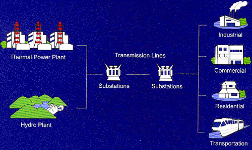
TNB customers are connected with power from hydroelectric and thermal plants through a network system made up of transmission lines, substations and distribution lines. It is via this reliable system that TNB supplies electricity to customers consistently and continuously, as well as ensuring a balance between demand and supply at all times.
The Unit Commitment Problem (UCP)
Every hour, electricity companies need to decide which power generators to run, in which periods and at what level in order to satisfy the demand for electricity. This problem is known as the Unit Commitment Problem (UCP).
The objective of the UCP is to optimize the electricity generation to cover the forecasted demand in accordance with fluctuating price forecasts and constraints on reservoir capacity of the different types of units.
The known characteristics of the generators usually are
- minimum and maximum capacity
- ramp-up and down capacity (how much more or less the generator can produce from one period to the next)
- availability, fixed cost of operating the generator
- variable cost of producing one unit of electricy per period
Predictive models are used to generate the demand forecast.
Thermal Power Plant
TNB’s Thermal Power Plant produces power by using conventional steam turbine and steam generator principally fired by coal, oil or natural gas (steam power plant), gas-fired or diesel-fired open cycle gas turbine generators, and gas-fired or diesel-fired combined cycle turbine generators.
A number of thermal power plants are committed to meeting the following electricity load demands over a day:
| Period | Begin | End | Demand (megawatts) |
|---|---|---|---|
| 1 | 0h | 4h | 5 000 |
| 2 | 4h | 8h | 10 000 |
| 3 | 8h | 12h | 25 000 |
| 4 | 12h | 16h | 30 000 |
| 5 | 16h | 20h | 40 000 |
| 6 | 20h | 0h | 27 000 |
There are five types of generating unit available. Each generator has to work between a minimum and a maximum level. There is an hourly cost of running each generator at minimum level. In addition there is an extra hourly cost for each megawatt at which a unit is operated above minimum level. To start up a generator also involves a cost. All this information is given in Table below (with costs in RM).
| Type | Minimum level (MW) | Maximum level (MW) | Cost per hour at minimum | Leveled cost per hour per megawatt above minimum (RM) | Startup Cost (RM) | Quantity |
|---|---|---|---|---|---|---|
| 1 | 800 | 1071 | 1200 | 3.47 | 1000 | 5 |
| 2 | 1200 | 2253 | 3000 | 3.53 | 2000 | 4 |
| 3 | 500 | 1000 | 1000 | 2.278 | 1500 | 8 |
| 4 | 400 | 1000 | 800 | 2.667 | 500 | 15 |
| 5 | 1000 | 1400 | 1500 | 3.74 | 1200 | 7 |
In addition to meeting the estimated load demands there must be sufficient generators working at any time to make it possible to meet an increase in load of up to 15%. This increase would have to be accomplished by adjusting the output of generators already operating within their permitted limits.
This problem is similar to that described by Garver (1963) [1], which involves scheduling electric generators to meet varying loads at different times of day.
The model estimates the lower cost of generating electricity within a given plan. Depending on the demand for electricity, we turn on or off units that generate power and which have operational properties and costs.
We will build a simple OPL/CPLEX model for the above UC problem to schedule power generators to meet demand.
Model Formulation
The following is the simple formulation.
The decision variables of are
- How many generators are turned on per time period?
- How much each unit produces per time period?
Demand must be met in each period.
\begin{aligned}
\sum_{i} P^p_i\ \geq\ d^p \quad \forall p \\
\end{aligned}
d^p is the Demand given in period p. P^p_i is the total output rate production from generators of type i in period p.
Production output must lie within the limits of the generators working.
\begin{aligned}
\underline{m}_i\ W^p_i \ \leq P^p_i \ \leq\ \overline{m}_i\ W^p_i \quad \forall i,p \\
\end{aligned}
W^p_i is the number of generating units of type i working in period p.
\underline{m}_i is the minimum output levels for generators of type i and \overline{m}_i is the maximum output levels for generators of type i.
The extra guranteed load requirement, g must be able to be met without starting up any more generators.
\begin{aligned}
\sum_i W^p_i\ \overline{m}_i  \geq (1 + g) * d^p \quad \forall p \\
\end{aligned}
The number of generators started in period p must equal the difference between the generators on at period p and at period p - 1. To avoid having to introduce an extra \max \lbrace 0, S \rbrace equation, the difference is written as an inequality. The objective function will enforce the equality
\begin{aligned}
S^p_i \geq W^p_i - W^{p- 1}_i & \quad \forall i, p \\
S^1_i = W^1_i & \quad \forall i\\
\end{aligned}
S^p_i is the number of generators of type i started up in period p.
All the integer variables have simple upper bounds corresponding to the total number of generators of each type, q_i.
\begin{aligned}
W^p_i \leq q_i \quad \forall i, p \\
\end{aligned}
Objective
Our objective is to decide which units should be working in which periods of the day to minimize total cost. The total cost is the total of startup cost, C, minimum cost per hour, c_i and level cost per hour, l_i for a period from begin, b^p to end, e^p.
\begin{aligned}
\min & \sum_p \sum_i l_i * (e_j - b_j) * (P^p_i - \underline{m}_i * W^p_i)\\
\ + & \sum_p \sum_i W^p_i * (e_j - b_j) * c_i\\
\ + & \sum_p \sum_i S^p_i * C_i\\
\end{aligned}
Modeling tricks
The reader may be surprised that the individual production of each unit is not computed. One could introduce variables w^p_{ik} \in \lbrace 0, 1 \rbrace for generator number k of type i and p^p_{ik} \in \mathbb{R}^+ the production for that generator
Then we would have
\underline{m}_i w^p_{ik} \leq p^p_{ik} \leq \overline{m}_i w^p_{ik}and
\begin{aligned}
& \sum_k w^p_{ik} = W^p_i\\
& \sum_k p^p_{ik} = P^p_i\\
\end{aligned}
But the w and p variables not appearing anywhere else (not in the objective function nor other constraints), they can be replaced by their summation. This is usually called a variable aggregation.
.mod
/*********************************************
 * OPL 12.10.0.0 Model
 * Author: diegoolivierfernandezpons
 * Creation Date: Oct 19, 2020 at 12:27:55 PM
 *********************************************/

 int nbGenerators = ...;
 int nbPeriods = ...;

 range generators = 1 .. nbGenerators;
 range periods = 1 .. nbPeriods;

 float qty [generators] = ...;
 float mn  [generators] = ...;
 float mx  [generators] = ...;
 float ch  [generators] = ...;
 float clh [generators] = ...;
 float cs  [generators] = ...;

 int begin  [periods] = ...;
 int end    [periods] = ...;
 float demand [periods] = ...;
 float r = ...;

 int dur [p in periods] = end[p] - begin[p];

 dvar int+   W [generators][periods];
 dvar float+ S [generators][periods];
 dvar float+ P [generators][periods];

 minimize
    sum (g in generators, p in periods) cs[g] * S[g][p] +
    sum (g in generators, p in periods) dur[p] * ch[g] * W[g][p] +
    sum (g in generators, p in periods) dur[p] * clh[g] * (P[g][p] - mn[g] * W[g][p]);

 constraints {

    // Cover the demand
    forall (p in periods) sum (g in generators) P[g][p] >= demand[p];

    // Cover the reserve
    forall (p in periods) sum (g in generators) mx[g] * W[g][p] >= (1 + r) * demand[p];

    // Production limits
    forall (g in generators, p in periods) mn[g] * W[g][p] <= P[g][p];
    forall (g in generators, p in periods) P[g][p] <= mx[g] * W[g][p];

    // Maximum number of generators
    forall (g in generators, p in periods) W[g][p] <= qty[g];

    // Start new generators
    forall (g in generators, p in periods : p - 1 in periods) S[g][p] >= W[g][p] - W[g][p - 1];
    forall (g in generators) S[g][1] == W[g][1];

 }
.dat
nbGenerators = 5;
qty = [5, 4, 8, 15, 7];
mn = [800, 1200, 500, 400, 1000];
mx = [1071, 2253, 1000, 1000, 1400];
ch = [1200, 3000, 1000, 800, 1500];
clh = [3.47, 3.53, 2.278, 2.667, 3.74];
cs = [1000, 2000, 1500, 500, 1200];

nbPeriods = 6;
begin = [0, 4, 8, 12, 16, 20];
end = [4, 8, 12, 16, 20, 24];
demand = [5000, 10000, 25000, 30000, 40000, 27000];
r = 0.15;
Result
The total daily cost of this operating pattern is RM 1,091,848.80
// solution (optimal) with objective 1091848.8
// Quality Incumbent solution:
// MILP objective                                 1.0918488000e+06
// MILP solution norm |x| (Total, Max)            1.37205e+05  1.50000e+04
// MILP solution error (Ax=b) (Total, Max)        0.00000e+00  0.00000e+00
// MILP x bound error (Total, Max)                0.00000e+00  0.00000e+00
// MILP x integrality error (Total, Max)          0.00000e+00  0.00000e+00
// MILP slack bound error (Total, Max)            0.00000e+00  0.00000e+00
//

S = [[0
             5 0 0 0 0]
             [0 0 0 4 0 0]
             [0 0 8 0 0 0]
             [0 0 15 0 0 0]
             [5 1 1 0 0 0]];
W = [[0 5 5 5 5 5]
             [0 0 0 4 4 2]
             [0 0 8 8 8 8]
             [0 0 15 15 15 15]
             [5 6 7 7 7 7]];
P = [[0 4000 4000 4000 5200 4000]
             [0 0 0 4800 4800 2400]
             [0 0 8000 8000 8000 7600]
             [0 0 6000 6200 15000 6000]
             [5000 6000 7000 7000 7000 7000]];
This UC model helps the electricity company to optimize the overall goals as possible.
CoEnzyme & CPLEX
CoEnzyme provides complete solutions for hydropower and mixed hydro/thermal generating planning based on IBM ILOG CPLEX Optimization engines and mathematical models.
Benefits / ROI:
- Enables energy utilities to deliver the least expensive rate to customers while still delivering the most reliable service possible
- Supports compliance with energy conservation and environmental protection regulations
- Reduces costs of operations through accurate capacity planning that reduces wear on generating equipment
References
[1] Garver, L. L. 1963. "Power scheduling by integer programming". IEEE Trans. Power Apparatus and Systems, 81, 730735.