Berth Allocation Problem (BAP)
The berth allocation problem assigns arriving ships to a section of the berth (where, when & how long) during enough time for the loading and unloading operations to take place.

Photo by Alex Duffy on Unsplash
We make the following assumptions and simplifications
- The berth is divided into sections of constant length, and a number of adjacent sections are simultaneously assigned to each berthed ship.
- Time is discrete and we assume a large enough planning horizon
- An average speed of container unloading is used to compute time needed to unload all the containers in a ship
- We ignore the number of cranes used for unloading containers, their location and their movements.
With these assumptions, the problem becomes a rectangle packing problem, which we will solve with IBM Cplex OPL Studio.
Rectangle Packing Problem
The rectangle packing is a packing problem where rectangle have to be packed in a larger rectangle without any overlap.
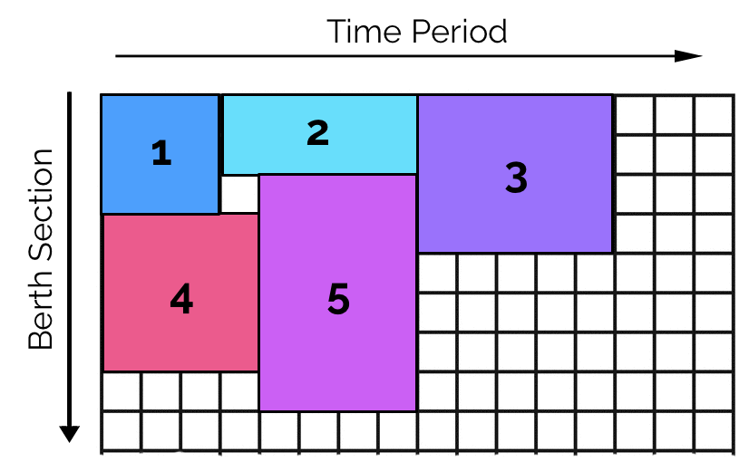
In the berth allocation problem, each ship is be represented by a rectangle where the length is its unloading time and its height is number of segments occupied in the berth.
| Ship | Unloading time | Berthing length |
|---|---|---|
| 1 | 3 | 3 |
| 2 | 5 | 2 |
| 3 | 5 | 4 |
| 4 | 4 | 4 |
| 5 | 4 | 6 |
Various objective functions are possible, we will minimize the total time taken to complete all the unloading tasks
Mathematical formulation
After assigning to each rectangle i a position defined by two floating point variables x_i and y_i, the next problem is to represent the non-overlap constraint. This is done by defining boolean variables that define for each pair (i, j) of rectangles whether i is on the left, right, above or below j. The link between the (x_i, y_i), (x_j, y_j) positions and the \text{left}_{ij}, \text{above}_{ij} variables is created using indicator constraints.
Indicator constraints are logic combinations of linear inequalities, which are automatically linearized by Cplex, but may also be linearized by hand if desired.
\begin{aligned}
& \quad \quad \min \max_i (x_i + W_i) & (1)\\
\\
& \forall ij \quad (l_{ij} = 1) \Leftrightarrow (x_i + W_i \leq x_j) & \quad (2)\\
& \forall ij \quad (a_{ij} = 1) \Leftrightarrow  (y_i + H_i \leq y_j) & \quad (3)\\
& \forall i < j \quad l_{ij} + l_{ji} + a_{ji} + a_{ji} \geq 1 & \quad (4)\\
& \forall i \quad x_i + W_i \leq W & \quad (5)\\
& \forall i \quad y_i + H_i \leq H & \quad (6)\\
\\
& \quad x_i\ y_i \in \mathbb{R}^+ &\\
& \quad l_i\ a_i \in \lbrace 0, 1  \rbrace &\\
\end{aligned}
The objective (1) minimizes the makespan of the assignment (the end of the last task). Constraints (2) and (3) define the boolean variable l_{ij} and a_{ij} as the indicator constraint that measures whether x_i + W_i \leq y_i. Equation (4) is the no-overlapping constraint and forces any par of rectangles to be either one on the left of the other, or one above the other. Constraints (5) and (6) ensure the rectangle remains within the admissible area.
Linearizaton of the indicator constraint
The indicator constraint may be linearized in various ways
\begin{aligned}
& x_i + W_i + W * l_{ij} \leq x_j + W\\
& x_i + l_{ij} * (W_i + W) \leq x_j + W\\
& x_i + W_i \leq x_j + (1 - l_{ij}) * W\\
\end{aligned}
In all cases when l_{ij} = 1 the inequality reduces to x_i + W_i \leq x_j and when l_{ij} = 0 the equation reduces to something that is always true.
However, the model running time may differ depending on the chosen linearization if any or the usage of an indicator constraint.
Improvements
Some improvements are easy to integrate in the model
Arrival times and waiting time
Arrival times just introduce extra bounds on the position variable x_i \geq R_i, which in turn allows a change in the objective to minimization of the maximum waiting time \min \max_i (x_i - R_i) or a minimization of the tardiness \min \sum_i (x_i + W_i - R_i)
Incompatibilities with berth positions
An incompatibility of a ship with some positions in the berth (because of insufficient depth for instance) creates a forbidden range of values for the y_i variable which can be represented by the constraint (y_i \leq L)\ ||\ (y_i \geq U). It is again a logic combination of linear constraints that can either be given directly to Cplex or linearized with the introduction of two boolean variables belowL and aboveU and the constraint b_L + a_U = 1
Lexicographic objective
Minimizing the makespan may result in solutions that are not completely "pushed to the left" because moving the yellow ship to an earlier time doesn’t change the end of the green ship.

A possible solution is to optimize lexicographically the makespan and the tardiness
dexpr float makespan = max (s in ships) (x[s] + ship_unloading_time[s]);
dexpr float tardiness = sum (s in ships) (x[s] + ship_unloading_time[s]);

minimize staticLex (makespan, tardiness);

constraints {
     ...
}
Which results in the following solution (results may vary)

Delays and stochastic optimization
Arrivals of ships as well as average loading times are estimations that may be wrong. Errors on average values are typically estimated with a probability distribution fitted to historical data – the most popular one being the normal distribution with parameters average \mu and deviation \sigma.
Stochastic optimization takes into account the fact that constants may deviate from their estimated average, and instead of optimizing over a single scenario, they optimize on expected value over a distribution of scenarios.
Cranes
Approximating the time it takes to unload the containers of a ship with an average is a very crude approximation as the number of cranes available on the berth is small, their mobility is limited, and the containers in the ship are located on multiple bays (positions along the berth).

Photo by Freddie on Unsplash
This justifies the interest in the combined berth assignment and crane scheduling problem which we will analyze in a subsequent blog post.
An OPL model
For simplicity we have chosen the OPL model with indicator variables. The reader may modify it to try any of the linearizations suggested – which in our tests reduce the running times of the model.
The reader is invited to add constraints to the model and experiment with it.
Model
/*********************************************
 * OPL 12.10.0.0 Model
 * Author: diegoolivierfernandezpons
 * Creation Date: Nov 11, 2020 at 2:58:22 PM
 *********************************************/

int number_of_ships = ...;

range ships = 1 .. number_of_ships;
int ship_length [ships] = ...;
int ship_unloading_time [ships] = ...;

int berth_length = ...;
int horizon = sum (s in ships) ship_unloading_time[s];

dvar float+ x[ships];
dvar float+ y[ships];

dexpr int left [i in ships][j in ships] = x[i] + ship_unloading_time[i] <= x[j];
dexpr int above [i in ships][j in ships] = y[i] + ship_length[i] <= y[j];

minimize max (s in ships) (x[s] + ship_unloading_time[s]);

constraints {

    // Non overlapping constraint
    forall(i, j in ships : i < j)
        left[i][j] + left[j][i] + above[i][j] + above[j][i] >= 1;

    // Ships within bounds
    forall (i in ships) x[i] + ship_unloading_time[i] <= horizon;
    forall (i in ships) y[i] + ship_length[i] <= berth_length - 1;
}
Data
berth_length = 10;
number_of_ships = 5;

ship_length = [3,2,4,4,6];
ship_unloading_time = [3,5,5,4,4];
Engine log
Version identifier: 12.10.0.0 | 2019-11-26 | 843d4de
CPXPARAM_TimeLimit                               300
Tried aggregator 2 times.
MIP Presolve eliminated 16 rows and 5 columns.
MIP Presolve modified 18 coefficients.
Aggregator did 23 substitutions.
Reduced MIP has 70 rows, 75 columns, and 182 nonzeros.
Reduced MIP has 41 binaries, 0 generals, 0 SOSs, and 25 indicators.
Presolve time = 0.00 sec. (0.17 ticks)
Probing changed sense of 2 constraints.
Probing time = 0.00 sec. (0.07 ticks)
Cover probing fixed 0 vars, tightened 6 bounds.
Tried aggregator 2 times.
MIP Presolve eliminated 2 rows and 2 columns.
Aggregator did 8 substitutions.
Reduced MIP has 60 rows, 65 columns, and 170 nonzeros.
Reduced MIP has 39 binaries, 0 generals, 0 SOSs, and 25 indicators.
Presolve time = 0.00 sec. (0.15 ticks)
Probing fixed 0 vars, tightened 2 bounds.
Probing time = 0.00 sec. (0.06 ticks)
Tried aggregator 1 time.
Detecting symmetries...
Reduced MIP has 60 rows, 65 columns, and 170 nonzeros.
Reduced MIP has 39 binaries, 0 generals, 0 SOSs, and 25 indicators.
Presolve time = 0.00 sec. (0.11 ticks)
Probing time = 0.00 sec. (0.05 ticks)
Clique table members: 30.
MIP emphasis: balance optimality and feasibility.
MIP search method: dynamic search.
Parallel mode: deterministic, using up to 4 threads.
Root relaxation solution time = 0.00 sec. (0.11 ticks)

        Nodes                                         Cuts/
   Node  Left     Objective  IInf  Best Integer    Best Bound    ItCnt     Gap

*     0+    0                           21.0000        9.0000            57.14%
      0     0        9.0000    23       21.0000        9.0000       16   57.14%
      0     0        9.0000    23       21.0000       Cuts: 8       22   57.14%
      0     0        9.0000    23       21.0000       Cuts: 7       29   57.14%
      0     0        9.0000    23       21.0000      Cuts: 22       41   57.14%
*     0+    0                           14.0000        9.0000            35.71%
      0     0        9.0000    23       14.0000      Cuts: 12       50   35.71%
*     0+    0                           13.0000        9.0000            30.77%
*     0+    0                           12.0000        9.0000            25.00%
Detecting symmetries...
      0     2        9.0000     6       12.0000        9.0000       50   25.00%
Elapsed time = 0.06 sec. (3.57 ticks, tree = 0.02 MB, solutions = 4)
*    10+    2                           11.0000        9.0000            18.18%

Clique cuts applied:  2
Cover cuts applied:  4
Implied bound cuts applied:  43
Mixed integer rounding cuts applied:  8
Gomory fractional cuts applied:  4

Root node processing (before b&c):
  Real time             =    0.05 sec. (3.53 ticks)
Parallel b&c, 4 threads:
  Real time             =    0.14 sec. (2.86 ticks)
  Sync time (average)   =    0.09 sec.
  Wait time (average)   =    0.00 sec.
                          ------------
Total (root+branch&cut) =    0.20 sec. (6.39 ticks)
Result
// solution (optimal) with objective 11
// Quality Incumbent solution:
// MILP objective                                 1.1000000000e+01
// MILP solution norm |x| (Total, Max)            1.04000e+02  1.10000e+01
// MILP solution error (Ax=b) (Total, Max)        0.00000e+00  0.00000e+00
// MILP x bound error (Total, Max)                0.00000e+00  0.00000e+00
// MILP x integrality error (Total, Max)          0.00000e+00  0.00000e+00
// MILP slack bound error (Total, Max)            0.00000e+00  0.00000e+00
// MILP indicator slack bound error (Total, Max)  0.00000e+00  0.00000e+00
//

x = [4 0 6 7 0];
y = [4 7 0 4 1];
References
[1] Ak, Aykagan. 2011. Berth and Quay Crane Scheduling: Problems, Models and Solution Methods (Book and PhD Thesis, Georgia Institute of Technology, Dec 2008).